Download
1 / 48
480 likes | 496 Views
Introduction to ROBOTICS. A Taste of Robot Localization Course Summary. Dr. John (Jizhong) Xiao Department of Electrical Engineering City College of New York jxiao@ccny.cuny.edu. Topics. Brief Review (Robot Mapping) A Taste of Localization Problem Course Summary. Mapping/Localization.

E N D
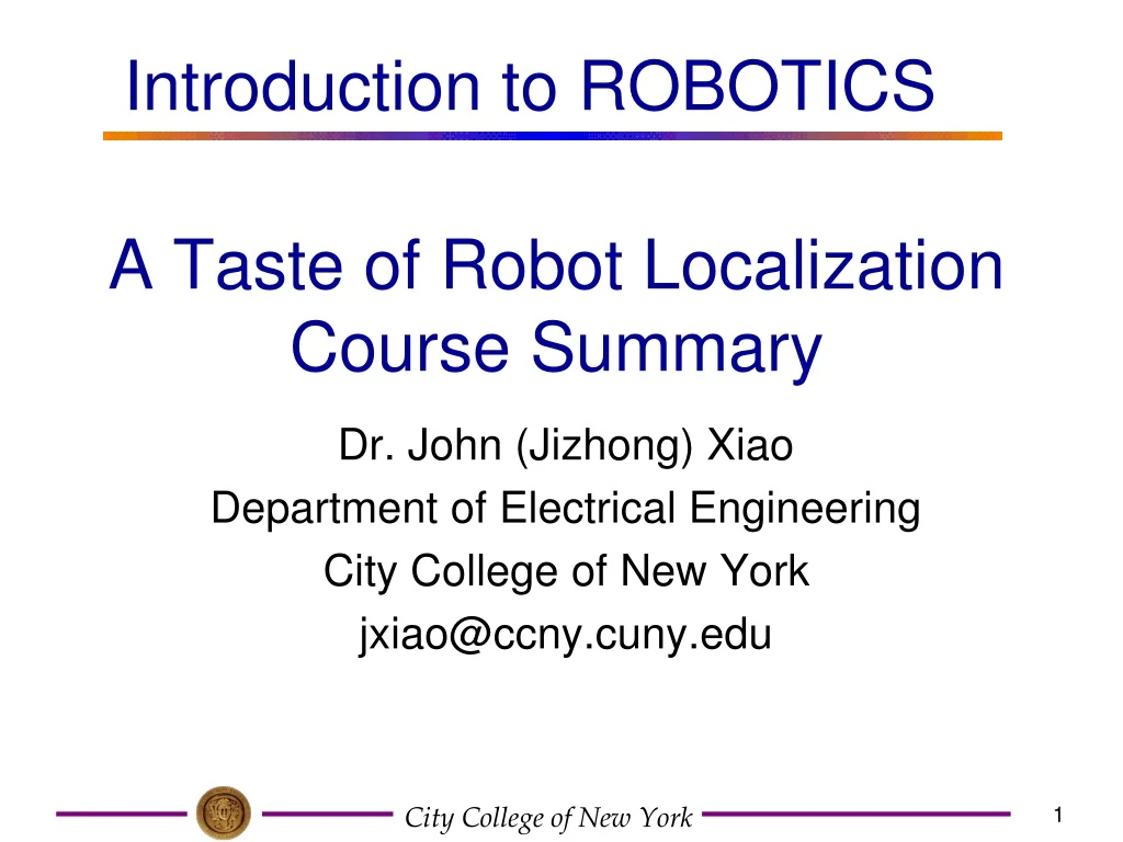
Introduction to ROBOTICS A Taste of Robot Localization Course Summary Dr. John (Jizhong) Xiao Department of Electrical Engineering City College of New York jxiao@ccny.cuny.edu
Topics • Brief Review (Robot Mapping) • A Taste of Localization Problem • Course Summary
Mapping/Localization • Answering robotics’ big questions • How to get a map of an environment with imperfect sensors (Mapping) • How a robot can tell where it is on a map (localization) • It is an on-going research • It is the most difficult task for robot • Even human will get lost in a building!
Review: Use Sonar to Create Map What should we conclude if this sonar reads 10 feet? there isn’t something here there is something somewhere around here 10 feet Local Map unoccupied no information occupied
What is it a map of? Several answers to this question have been tried: cell (x,y) is unoccupied cell (x,y) is occupied oxy oxy It’s a map of occupied cells. pre ‘83 What information should this map contain, given that it is created with sonar ? Each cell is either occupied or unoccupied -- this was the approach taken by the Stanford Cart.
What is it a map of ? Several answers to this question have been tried: cell (x,y) is unoccupied cell (x,y) is occupied oxy oxy It’s a map of occupied cells. It’s a map of probabilities: p( o | S1..i ) p( o | S1..i ) pre ‘83 The certainty that a cell is occupied, given the sensor readings S1, S2, …, Si ‘83 - ‘88 The certainty that a cell is unoccupied, given the sensor readings S1, S2, …, Si The odds of an event are expressed relative to the complement of that event. It’s a map of odds. evidence = log2(odds) probabilities p( o | S1..i ) odds( o | S1..i ) = The odds that a cell is occupied, given the sensor readings S1, S2, …, Si p( o | S1..i )
So, how do we combine evidence to create a map? What we want -- the new value of a cell in the map after the sonar reading S2 odds( o | S2 S1) What we know -- the old value of a cell in the map (before sonar reading S2) odds( o | S1) the probabilities that a certain obstacle causes the sonar reading Si p( Si | o ) & p( Si | o ) Combining Evidence • The key to making accurate maps is combining lots of data.
Combining Evidence • The key to making accurate maps is combining lots of data. p( o | S2 S1 ) def’n of odds odds( o | S2 S1) = p( o | S2 S1 ) p( S2 S1 | o) p(o) . = Bayes’ rule (+) p( S2 S1 | o) p(o) p( S2 | o) p( S1 | o) p(o) conditional independence of S1 and S2 . = p( S2 | o) p( S1 | o) p(o) p( S2 | o) p( o | S1 ) Bayes’ rule (+) . = p( S2 | o) p( o | S1 ) previous odds precomputed values the sensor model Update step = multiplying the previous odds by a precomputed weight.
Mapping Using Evidence Grids Evidence Grids... represent space as a collection of cells, each with the odds (or probability) that it contains an obstacle evidence = log2(odds) Lab environment likely free space likely obstacle lighter areas: lower evidence of obstacles being present not sure darker areas: higher evidence of obstacles being present
high-level Motion Planning: Given a known world and a cooperative mechanism, how do I get there from here ? Localization: Given sensors and a map, where am I ? Vision: If my sensors are eyes, what do I do? Mapping: Given sensors, how do I create a useful map? Abstraction level Bug Algorithms: Given an unknowable world but a known goal and local sensing, how can I get there from here? Kinematics: if I move this motor somehow, what happens in other coordinate systems ? Control (PID): what voltage should I set over time ? low-level Motor Modeling: what voltage should I set now ? Mobot System Overview
Content • Brief Review (Robot Mapping) • A Taste of Localization Problem • Course Summary
What’s the problem? • WHERE AM I? • But what does this mean, really? • Frame of reference is important • Local/Relative: Where am I vs. where I was? • Global/Absolute: Where am I relative to the world frame? • Location can be specified in two ways • Geometric: Distances and angles • Topological: Connections among landmarks
Localization: Absolute • Proximity-To-Reference • Landmarks/Beacons • Angle-To-Reference • Visual: manual triangulation from physical points • Distance-From-Reference • Time of Flight • RF: GPS • Acoustic: • Signal Fading • EM: Bird/3Space Tracker • RF: • Acoustic:
Triangulation Land Landmarks Works great -- as long as there are reference points! Lines of Sight Unique Target Sea
Compass Triangulation cutting-edge 12th century technology Land Landmarks Lines of Sight North Unique Target Sea
Localization: Relative • If you know your speed and direction, you can calculate where you are relative to where you were (integrate). • Speed and direction might, themselves, be absolute (compass, speedometer), or integrated (gyroscope, Accelerometer) • Relative measurements are usually more accurate in the short term -- but suffer from accumulated error in the long term • Most robotics work seems to focus on this.
Localization Methods • Markov Localization: • Represent the robot’s belief by a probability distribution over possible positions and uses Bayes’ rule and convolution to update the belief whenever the robot senses or moves • Monte-Carlo methods • Kalman Filtering • SLAM (simultaneous localization and mapping) • ….
Markov Localization • What is Markov Localization ? • Special case of probabilistic state estimation applied to mobile robot localization • Initial Hypothesis: • Static Environment • Markov assumption • The robot’s location is the only state in the environment which systematically affects sensor readings • Further Hypothesis • Dynamic Environment
Markov Localization • Instead of maintaining a single hypothesis as to where the robot is, Markov localization maintains a probability distribution over the space of all such hypothesis • Uses a fine-grained and metric discretization of the state space
Example • Assume the robot position is one- dimensional The robot is placed somewhere in the environment but it is not told its location The robot queries its sensors and finds out it is next to a door
Example The robot moves one meter forward. To account for inherent noise in robot motion the new belief is smoother The robot queries its sensors and again it finds itself next to a door
Basic Notation Bel(Lt=l ) Is the probability (density) that the robot assigns to the possibility that its location at time t is l The belief is updated in response to two different types of events: • sensor readings, • odometry data
Notation • Goal:
Update Phase a b c
Markov Localization • Topological (landmark-based, state space organized according to the topological structure of the environment) • Grid-Based (the world is divided in cells of fixed size; resolution and precision of state estimation are fixed beforehand) • The latter suffers from computational overhead
Content • Brief Review (Robot Mapping) • A Taste of Localization Problem • Course Summary
R Mobile Robot Locomotion Locomotion: the process of causing a robot to move • Differential Drive • Tricycle Swedish Wheel • Synchronous Drive • Ackerman Steering • Omni-directional
Differential Drive Property: At each time instant, the left and right wheels must follow a trajectory that moves around the ICC at the same angular rate , i.e., • Kinematic equation • Nonholonomic Constraint
Differential Drive • Basic Motion Control • R : Radius of rotation • Straight motion • R = Infinity VR = VL • Rotational motion • R = 0 VR = -VL
Tricycle • Steering and power are provided through the front wheel • control variables: • angular velocity of steering wheel ws(t) • steering direction α(t) d: distance from the front wheel to the rear axle
Tricycle Kinematics model in the world frame ---Posture kinematics model
Synchronous Drive • All the wheels turn in unison • All wheels point in the same direction and turn at the same rate • Two independent motors, one rolls all wheels forward, one rotate them for turning • Control variables (independent) • v(t), ω(t)
R Ackerman Steering (Car Drive) • The Ackerman Steering equation: • :
ICC Y R l X Car-like Robot Driving type: Rear wheel drive, front wheel steering Rear wheel drive car model: : forward velocity of the rear wheels : angular velocity of the steering wheels non-holonomic constraint: l :length between the front and rear wheels
Robot Sensing • Collect information about the world • Sensor - an electrical/mechanical/chemical device that maps an environmental attribute to a quantitative measurement • Each sensor is based on a transduction principle - conversion of energy from one form to another • Extend ranges and modalities of Human Sensing
Gas Sensor Gyro Accelerometer Metal Detector Pendulum Resistive Tilt Sensors Piezo Bend Sensor Gieger-Muller Radiation Sensor Pyroelectric Detector UV Detector Resistive Bend Sensors CDS Cell Resistive Light Sensor Digital Infrared Ranging Pressure Switch Miniature Polaroid Sensor Limit Switch Touch Switch Mechanical Tilt Sensors IR Sensor w/lens IR Pin Diode Thyristor Magnetic Sensor Polaroid Sensor Board Hall Effect Magnetic Field Sensors Magnetic Reed Switch IR Reflection Sensor IR Amplifier Sensor IRDA Transceiver IR Modulator Receiver Radio Shack Remote Receiver Lite-On IR Remote Receiver Solar Cell Compass Compass Piezo Ultrasonic Transducers
Sensors Used in Robot • Resistive sensors: • bend sensors, potentiometer, resistive photocells, ... • Tactile sensors: contact switch, bumpers… • Infrared sensors • Reflective, proximity, distance sensors… • Ultrasonic Distance Sensor • Motor Encoder • Inertial Sensors (measure the second derivatives of position) • Accelerometer, Gyroscopes, • Orientation Sensors: Compass, Inclinometer • Laser range sensors • Vision, GPS, …
Motion Planning Path Planning: Find a path connecting an initial configuration to goal configuration without collision with obstacles • Configuration Space • Motion Planning Methods • Roadmap Approaches • Cell Decomposition • Potential Fields • Bug Algorithms
Motion Planning • Motion Planning Methodololgies • – Roadmap • – Cell Decomposition • – Potential Field • • Roadmap • – From Cfree a graph is defined (Roadmap) • – Ways to obtain the Roadmap • • Visibility graph • • Voronoi diagram • • Cell Decomposition • – The robot free space (Cfree) is decomposed into simple regions (cells) • – The path in between two poses of a cell can be easily generated • • Potential Field • – The robot is treated as a particle acting under the influence of a potential field U, • where: • • the attraction to the goal is modeled by an additive field • • obstacles are avoided by acting with a repulsive force that yields a negative field Global methods Local methods
Full-knowledge motion planning Roadmaps Cell decompositions visibility graph exact free space represented via convex polygons voronoi diagram approximate free space represented via a quadtree
Potential field Method • Usually assumes some knowledge at the global level The goal is known; the obstacles sensed Each contributes forces, and the robot follows the resulting gradient.
Thank you! Next Week: Final Exam Time: Dec. 13, 6:30pm-9:00pm, Place: T512 Coverage: Mobile Robot, Close-book with 1 page cheat sheet