Download
1 / 13
130 likes | 245 Views
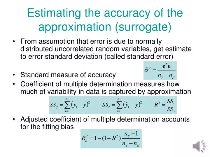
Estimating the accuracy of the approximation (surrogate). From assumption that error is due to normally distributed uncorrelated random variables, get estimate to error standard deviation (called standard error) Standard measure of accuracy

E N D
Estimating the accuracy of the approximation (surrogate) • From assumption that error is due to normally distributed uncorrelated random variables, get estimate to error standard deviation (called standard error) • Standard measure of accuracy • Coefficient of multiple determination measures how much of variability in data is captured by approximation • Adjusted coefficient of multiple determination accounts for the fitting bias
Curve fit • noise=randn(1,30); x=1:1:30; y=x+noise • 3.908 2.825 4.379 2.942 4.5314 5.7275 8.098 …………………………………25.84 27.47 27.00 30.96 • [p,s]=polyfit(x,y,1); yfit=polyval(p,x); plot(x,y,'+',x,x,'r',x,yfit,'b') With dense data, functional form is clear. Fit serves to filter out noise
Example with y=0.1*x • noise=randn(1,30); x=1:1:30; y=0.1*x+noise; • xx=[ones(30,1),x']; [B,BINT,R,RINT,STATS] = regress(y',xx) • Stat 0.3016 12.0896 0.0017 1.7498
Estimating error in coefficients • Some coefficients are more accurately estimated than others • Standard error in coefficient is • t-statistic is ratio of coefficient to standard error, would like it to be at least 2 • Coefficients that are poorly estimated may be dropped to improve accuracy of predictions • Dropping one coefficients changes t-statistics for others • Need to iterate in dropping and adding coefficients
Example 3.2.1 • Given data • Use Microsoft Excel to fit linear and quadratic polynomials • Compare standard errors and t-statistics of coefficients
Cross validation • Error estimates based on model assumptions are vulnerable • For polynomial response surface approximations assumptions are rarely satisfied • Cross validation divides data into ng groups • Fit the approximation to ng -1 groups, and use last group to estimate error. Repeat for each group • When each group consists of one point, error called PRESS (prediction error sum of squares) • Calculate error at each point and then presenting r.m.s error • Can be shown that • Can be used only if not ill-conditioned
Questions • The pairs (0,0), (1,1), (2,1) represent strain (millistrains) and stress (ksi) measurements. • Estimate Young modulus using the three commonly used error norms. • Estimate the error in Young modulus using cross validation