Download
1 / 42
420 likes | 552 Views
4.1 introduction 4.2 virtual circuit and datagram networks 4.3 what ’ s inside a router 4.4 IP: Internet Protocol datagram format IPv4 addressing ICMP IPv6. 4.5 routing algorithms link state distance vector hierarchical routing 4.6 routing in the Internet RIP OSPF BGP

E N D
4.1 introduction 4.2 virtual circuit and datagram networks 4.3 what’s inside a router 4.4 IP: Internet Protocol datagram format IPv4 addressing ICMP IPv6 4.5 routing algorithms link state distance vector hierarchical routing 4.6 routing in the Internet RIP OSPF BGP 4.7 broadcast and multicast routing Chapter 4: outline Network Layer
routing algorithm determines end-end-path through network forwarding table determines local forwarding at this router 1 3 2 Interplay between routing, forwarding routing algorithm local forwarding table dest address output link address-range 1 address-range 2 address-range 3 address-range 4 3 2 2 1 IP destination address in arriving packet’s header Network Layer
5 3 5 2 2 1 3 1 2 1 z x w u y v Graph abstraction graph: G = (N,E) N = set of routers = { u, v, w, x, y, z } E = set of links ={ (u,v), (u,x), (v,x), (v,w), (x,w), (x,y), (w,y), (w,z), (y,z) } Network Layer
5 3 5 2 2 1 3 1 2 1 z x w u v y Graph abstraction: costs c(x,x’) = cost of link (x,x’) e.g., c(w,z) = 5 cost is inversely related to bandwidth, or proportionally related to congestion - high bandwidth, low congestion: cost 1 - low bandwidth, high congestion: high cost cost of path (x1, x2, x3,…, xp) = c(x1,x2) + c(x2,x3) + … + c(xp-1,xp) key question: what is the least-cost path between u and z ? routing algorithm: algorithm that finds that least cost path Network Layer
[Classification 1] Global or decentralized information? Global: all routers have complete topology and link cost info. “link state (LS)” algorithms Decentralized: router only knows physically-connected neighbors and link costs to neighbors iterative process of computation, exchange of info with neighbors “distance vector (DV)” algorithms Routing Algorithm classification Network Layer
[Classification 2] Static or dynamic? Static: Manual setup Network administrator usually setups the route routes does not change, or change slowly over time Dynamic: routes change more quickly periodic update in response to link cost changes LS and DV algorithms Routing Algorithm classification Network Layer
Routing Algorithm classification Static routing • Manually configuration routing table • Single “permanent” route is configured for each source to destination pair • Routes usually determined using a least cost algorithm • Route fixed, at least until a change in network topology • Can’t react dynamically to network change such as router’s crash • Practically, fixed routing is much used within an AS
Routing Algorithm classification Dynamic route • Network protocol adjusts automatically for topology or traffic changes • Unix hosts can run routing daemon routed or gated Routing Table Routing Table Routing Protocol Routing Protocol Update Routing Information
[Classification 3] Source or Hop-by-Hop? Source routing: Source will determine the entire route Routers only act as store-forward devices Hop-by-hop: Routers determine the path based on theirs’ own information LS and DV algorithms Routing Algorithm classification Network Layer
4.1 introduction 4.2 virtual circuit and datagram networks 4.3 what’s inside a router 4.4 IP: Internet Protocol datagram format IPv4 addressing ICMP IPv6 4.5 routing algorithms link state distance vector hierarchical routing 4.6 routing in the Internet RIP OSPF BGP 4.7 broadcast and multicast routing Chapter 4: outline Network Layer
Flooding “Link State” • Each node floods “link status” to the entire routers • Packet sent by source router to every neighbor • Incoming packet resent to all outgoing links except source link • Duplicate packets already transmitted are discarded • Prevent endless retransmission • All routers get information to build routing table • High traffic load • Use the link state to build a shortest path map to every node • Also known as Shortest Path First (SPF) algorithm Network Layer
Link State Algorithm - Overview • Exchange its connection and cost to its neighbors • Each router computes the set of optimum path to all destination (using a Shortest Path - Dijkstra's algorithm) X Z W Y link state link state link state Network Layer
Link State Algorithm - Overview • Each router initially begins with directly connected network • Determine full knowledge of distant routers and their connection R1 exchange link state packets R2 R4 build topological database Routing Table R3 compute SPF update routing table Network Layer
topology change Link State Algorithm - Overview • On the topology change, send the change information to other routers • Fast convergence R1 R4 R2 R3 Network Layer
Dijkstra’s algorithm net topology, link costs known to all nodes accomplished via “link state flooding (broadcast)” all nodes have same info computes the least cost paths from one node (‘source”) to all other nodes gives forwarding table for that node iterative: after k iterations, know least cost path to k destinations. notation: c(x,y): link cost from node x to y; = ∞ if not direct neighbors D(v): current value of cost of path from source to dest. V p(v): predecessor node along path from source to v N': set of nodes whose least cost path definitively known A Link-State Routing Algorithm Network Layer
5 3 5 2 2 1 3 1 2 1 x z w y u v value value value value value value link cost link cost link cost link cost link cost link cost ∞ 2 5 1 2 ∞ c(v,u) c(w,u) c(y,u) c(z,u) c(u,v) c(x,u) 2 2 ∞ 1 ∞ 3 c(y,v) c(z,v) c(w,v) c(x,v) c(v,x) c(u,x) c(y,x) c(x,y) c(z,x) c(u,y) c(v,y) c(w,x) ∞ ∞ 3 1 1 ∞ 5 3 1 1 2 3 c(z,y) c(u,w) c(x,w) c(w,y) c(y,w) c(v,w) c(u,z) c(x,z) c(y,z) c(w,z) c(z,w) c(v,z) 5 ∞ ∞ ∞ 5 2 Dijsktra’s Algorithm (see this, not one in the book) Inside node u 0 Pre-calculation: Network Layer
5 3 5 2 2 1 3 1 2 1 x z w y u v Dijsktra’s Algorithm (see this, not one in the book) Inside node u 1 Initialization: 2 N' = {u} 3 for all nodes v 4 if v adjacent to u 5 then D(v) = c(u,v) 6 else D(v) = ∞ 7 8 Loop 9 find e not in N' such that D(e) is a minimum 10 add e to N' 11 update D(n) for all n (not in N') adjacent to e: 12 D(n) = min( D(n), D(e) + c(e,n) ) 13 /* new cost to n is either old cost to n or known 14 shortest path cost to e plus cost from e to n */ 15 until all nodes in N' Network Layer
5 3 5 2 2 1 3 1 2 1 z x w u y v Dijkstra’s algorithm: example D(v),p(v) 2,u 2,u 2,u D(x),p(x) 1,u D(w),p(w) 5,u 4,x 3,y 3,y D(y),p(y) ∞ 2,x Step 0 1 2 3 4 5 N' u ux uxy uxyv uxyvw uxyvwz D(z),p(z) ∞ ∞ 4,y 4,y 4,y D(n) = min( D(n), D(e) + c(e,n) ) [Example] Step1: D(w) = min(D(w), D(x) + c(x,w)) = min(5, 1 + 3) = 4 D(y) = min(D(y), D(x) + c(x,y)) = min(∞, 1 + 1) = 2 Step2: D(w) = min(D(w), D(y) + c(y,w)) = min(4, 2 + 1) = 3 Network Layer
z x w u y v destination link (u,v) v (u,x) x y (u,x) (u,x) w z (u,x) Dijkstra’s algorithm: example resulting shortest-path tree from u: “resulting forwarding table” in u: Network Layer
Dijkstra’s algorithm: another example 9 11,w 14,x 11,w ∞ ∞ ∞ 3,u 5,u 5,u 6,w 6,w 7,u 7 5 4 8 3 w u x v y z 2 3 4 7 10,v 14,x D(v) p(v) D(w) p(w) D(x) p(x) D(y) p(y) D(z) p(z) Step N' u 0 uw 1 uwx 2 uwxv 3 uwxvy 4 12,y uwxvyz 5 notes: • construct shortest path tree by tracing predecessor nodes • ties can exist (can be broken arbitrarily) Network Layer
algorithm complexity:n nodes each iteration: need to check all nodes, w, not in N n(n+1)/2 comparisons: O(n2) more efficient implementations possible: O(nlogn) oscillations possible: e.g., support link cost equals amount of carried traffic: 2+e 0 0 0 1 1+e C C C C D D D D B B A B B A A A 2+e 2+e 0 0 1 1 1+e 1+e 0 0 0 0 given these costs, find new routing…. resulting in new costs given these costs, find new routing…. resulting in new costs given these costs, find new routing…. resulting in new costs Dijkstra’s algorithm, discussion 1 1+e 0 0 e 0 1 1 e initially Network Layer
4.1 introduction 4.2 virtual circuit and datagram networks 4.3 what’s inside a router 4.4 IP: Internet Protocol datagram format IPv4 addressing ICMP IPv6 4.5 routing algorithms link state distance vector hierarchical routing 4.6 routing in the Internet RIP OSPF BGP 4.7 broadcast and multicast routing Chapter 4: outline Network Layer
Distance vector algorithm At Node x, for the destination y via all other neighbor nodes let dx(y) := cost of least-cost path from x to y then dx(y) = min {c(x,v) + dv(y) } a, 22.7 b, 28.1 c, 15.1 dx(y) = where a, b, c are the neighbors Bellman-Ford equation (dynamic programming) v cost from neighbor v to destination y cost to neighbor v min taken over all neighbors v of x Network Layer
5 3 5 2 2 1 3 1 2 1 z x w u v y Bellman-Ford example Assume that router u knows… dv(z) = 5, dx(z) = 3, dw(z) = 3 B-F equation says: du(z) = min { c(u,v) + dv(z), c(u,x) + dx(z), c(u,w) + dw(z) } = min {2 + 5, 1 + 3, 5 + 3} = 4 “node achieving minimum” is the next hop in shortest path, used inforwarding table Network Layer
Distance vector algorithm • Dx(y) = estimate of least cost from x to y • x maintains “distance vector” Dx = [Dx(y): y є N ] • node x: • knows “exact” cost to each neighbor v: c(x,v) • maintains its neighbors’ distance vectors. • For each neighbor v, x maintains Dv = [Dv(y): y є N ] Network Layer
Distance vector algorithm key idea: • from time-to-time, each node sends its own distance vector (DV) estimate to neighbors • when x receives new DV estimate from neighbor, it updates its own DV using B-F equation: Dx(y) ← minv{c(x,v) + Dv(y)} for each node y ∊ N • under natural conditions, the estimate Dx(y) will converge to the actual cost dx(y) Network Layer
iterative, asynchronous:each local iteration caused by: local link cost change DV update message from neighbor distributed: each node notifies neighbors only when its DV changes neighbors then notify their neighbors if necessary Distance vector algorithm each node: waitfor (change in local link cost or msg from neighbor) recompute estimates if DV to any dest has changed, notify neighbors Network Layer
2 1 7 z y x Dx(z) = min{c(x,y) + Dy(z), c(x,z) + Dz(z)} = min{2+1 , 7+0} = 3 Dx(y) = min{c(x,y) + Dy(y), c(x,z) + Dz(y)} = min{2+0 , 7+1} = 2 node x table cost to cost to x y z x y z x 0 2 7 x 0 3 2 y y 2 0 1 from ∞ ∞ ∞ from z z 7 1 0 ∞ ∞ ∞ node y table cost to x y z x ∞ ∞ ∞ 2 0 1 y from z ∞ ∞ ∞ node z table cost to x y z x ∞ ∞ ∞ y from ∞ ∞ ∞ z 7 1 0 time Network Layer
2 1 7 z y x Dx(z) = min{c(x,y) + Dy(z), c(x,z) + Dz(z)} = min{2+1 , 7+0} = 3 Dx(y) = min{c(x,y) + Dy(y), c(x,z) + Dz(y)} = min{2+0 , 7+1} = 2 node x table cost to cost to cost to x y z x y z x y z x 0 2 7 x 0 3 2 x 0 2 3 y y 2 0 1 from ∞ ∞ ∞ y from 2 0 1 from z z 7 1 0 ∞ ∞ ∞ z 3 1 0 node y table cost to cost to cost to x y z x y z x y z x ∞ ∞ x 0 2 7 ∞ 2 0 1 x 0 2 3 y y 2 0 1 y from from 2 0 1 from z z ∞ ∞ ∞ 7 1 0 z 3 1 0 cost to cost to node z table cost to x y z x y z x y z Dz(x) = min{c(z,x) + Dx(x), c(z,y) + Dy(x)} = min{7+0 , 1+2} = 3 x 0 2 7 x 0 2 3 x ∞ ∞ ∞ y y 2 0 1 from y 2 0 1 from from ∞ ∞ ∞ z z z 3 1 0 3 1 0 7 1 0 time time Network Layer
SKIP!! 1 4 1 50 x z y Distance vector: link cost changes link cost changes: • node detects local link cost change • updates routing info, recalculates distance vector • if DV changes, notify neighbors t0 : y detects link-cost change, updates its DV, informs its neighbors. “good news travels fast” t1 : z receives update from y, updates its table, computes new least cost to x , sends its neighbors its DV. t2 : y receives z’s update, updates its distance table. y’s least costs do not change, so y does not send a message to z. Network Layer
SKIP!! 60 4 1 50 x z y Distance vector: link cost changes link cost changes: • node detects local link cost change • bad news travels slow - “count to infinity” problem! • 44 iterations before algorithm stabilizes At time t0, y detects the link-cost change, updates its DV, and informs its neighbors. Dy(x) = min{c(y,x)+Dx(x), c(y,z)+Dz(x)} = min{60+0, 1+5} = 6 “Routing Loop” occurs (from y to x: y send to z and z send to y) At time t1, z receives the update from y and updates its table. Dz(x) = min{c(z,x)+Dx(x), c(z,y)+Dy(x)} = min{50+0, 1+6} = 7 It computes a new least cost to x and sends its neighbors its DV. At time t2, y receives z’s update and updates its DV, and inform its neighbor Dy(x) = min{c(y,x)+Dx(x), c(y,z)+Dz(x)} = min{60+0, 1+7} = 8 … … Network Layer
SKIP!! 60 4 1 50 x z y Distance vector: link cost changes poisoned reverse: • If Z routes through Y to get to X : • Z tells Y its (Z’s) distance to X is infinite (so Y won’t route to X via Z) • will this completely solve count to infinity problem? Network Layer
message complexity LS: with n nodes, E links, O(nE) msgs sent Link State Flooding Fast Convergence DV:exchange between neighbors only convergence time varies (and slow) speed of convergence LS: O(n2) algorithm requires O(nE) msgs fast may have oscillations DV: convergence time varies (and slow) may be routing loops count-to-infinity problem robustness: what happens if router malfunctions? LS: node can advertise incorrect link cost each node computes only its own table DV: DV node can advertise incorrect path cost each node’s table used by others error propagate thru network Comparison of LS and DV algorithms Network Layer
4.1 introduction 4.2 virtual circuit and datagram networks 4.3 what’s inside a router 4.4 IP: Internet Protocol datagram format IPv4 addressing ICMP IPv6 4.5 routing algorithms link state distance vector hierarchical routing 4.6 routing in the Internet RIP OSPF BGP 4.7 broadcast and multicast routing Chapter 4: outline Network Layer
scale: with 600 million destinations: can’t store all dest’s in routing tables! routing table exchange would swamp links! administrative autonomy internet = network of networks each network admin may want to control routing in its own network Hierarchical routing our routing study thus far - idealization • all routers identical • network “flat” … not true in practice Network Layer
aggregate routers into regions,“autonomous systems (AS) ” routers in same AS run same routing protocol “intra-AS” routing protocol routers in different AS can run different intra-AS routing protocol gateway router: at “edge” of its own AS has link to router in another AS Hierarchical routing Network Layer
forwarding table configured by both intra- and inter-AS routing algorithm intra-AS sets entries for internal dests inter-AS & intra-AS sets entries for external dests 3a 3b 2a AS3 AS2 1a 2c AS1 2b 1b 1d 3c 1c Inter-AS Routing algorithm Intra-AS Routing algorithm Forwarding table Interconnected ASes Network Layer
suppose router in AS1 receives datagram destined outside of AS1: router should forward packet to gateway router, but which one? AS1 must: learn which dests are reachable through AS2, which through AS3 propagate this reachability info to all routers in AS1 job of inter-AS routing! 2c 2b 1b 1d 3c 1c 3a 3b 2a 1a AS1 Inter-AS tasks AS3 other networks other networks AS2 Network Layer
2c 2b 1b 1d 1c 3c 3a 3b 2a 1a AS1 Example: setting forwarding table in router 1d • suppose AS1 learns (via inter-AS protocol) that subnet x reachable via AS3 (gateway 1c), but not via AS2 • inter-AS protocol propagates reachability info to all internal routers • router 1d determines from intra-AS routing info that its interface I is on the least cost path to 1c • installs forwarding table entry (x,I) … x AS3 other networks other networks AS2 I Network Layer
2c 2b 1b 1d 1c 3c 3a 3b 2a 1a AS1 Example: choosing among multiple ASes • now suppose AS1 learns from inter-AS protocol that subnet x is reachable from AS3 and from AS2. • to configure forwarding table, router 1d must determine which gateway it should forward packets towards for dest x • this is also job of inter-AS routing protocol! … x …… AS3 other networks other networks AS2 ? Network Layer
Example: choosing among multiple ASes • now suppose AS1 learns from inter-AS protocol that subnet xis reachable from AS3 and from AS2. • to configure forwarding table, router 1d must determine towards which gateway it should forward packets for dest x • this is also job of inter-AS routing protocol! • hot potato routing: send packet towards the closest of two routers. determine from forwarding table the interface I that leads to least-cost gateway. Enter (x,I) in forwarding table use routing info from intra-AS protocol to determine costs of least-cost paths to each of the gateways learn from inter-AS protocol that subnet x is reachable via multiple gateways hot potato routing: choose the gateway that has the smallest least cost Network Layer
IGP IGP IGP IGP IGP IGP IGP IGP IGP Internet Routing Architecture IGP: Interior Gateway Protocols - RIP, OSPF, IGRP EGP: Exterior Gateway Protocols - BGP(Boarder Gateway Protocol) Autonomous System EGP/BGP EGP/BGP Autonomous System BGP4 BGP4 Autonomous System BGP4 Autonomous System EGP/BGP EGP/BGP EGP/BGP EGP/BGP Autonomous System Network Layer