Download
1 / 26
290 likes | 592 Views
Probability Distributions, the Law of Large Numbers and the Central Limit Theorem. Compare theoretical probability with a single sample and with many samples. Dale Nelson Salt Lake Community College November 2013.

E N D
Probability Distributions,the Law of Large Numbersand theCentral Limit Theorem Compare theoretical probability with a single sample and with many samples. Dale Nelson Salt Lake Community College November 2013
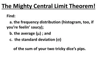
Part I. Theoretical ProbabilityUse the theoretical probability distribution for the results of the spinner to calculate the expected value, the standard deviation, and to make a histogram.
The expected value, or mean, of a probability distribution is EV = m = • The standard deviation: s =
Using an Excel spreadsheet to find the expected value, enter the title “x” in cell A1, and the values in cells A2 through A6 below. • Enter the title “P(x)” in cell B1 and the values in cells B2 through B6 below. • Enter the title “x.P(x)” in cell C1 and the function “=A2*B2” in cell C2. “Hook” the cell in the lower right corner and drag the function through to cell C6. • In cell C7 enter the function “=sum(C2:C6)”.
To use the spreadsheet to find the standard deviation, enter the title “x^2*P(x)” in cell D1, and the function “=A2^2*B2” in cells D2. “Hook” the cell and drag the function through to cell D6. • In cell D7 enter the function “=sum(D2:D6)”. • Enter the title “st. dev. =” in cell A8 and in cell B9 enter the function”=sqrt(D7-C7^2) • Give titles to the work done as shown below.
To make the probability histogram, highlight cells B2:B6, click the Insert tab, then select Column in the Charts section. Finally click the most basic choice in the upper left corner. Titles should be added to this using the Layout tab in the Chart Tools.
Part II : Single sample of size n = 25 • Use the Data Analysis program in the Analysis section of the Data tab to create a random sample. If it’s not there, it should be Added-In using the Analysis ToolPak . If using a Mac, I’ve heard there’s a free download available by Googling “StatPlus:mac”.
In the Data Analysis program, click Random Number Generation and enter the following Number of variables: 1 Number of random numbers: 25 Distribution: Discrete Value and Probability Range: A2:B6 Random seed: 0 < n < 32,767 Output Range: G1 The column of numbers generated represents 25 random spins.
Using the Excel spreadsheet, find the mean and standard deviation of the sample. Enter the title “mean =” in cell F26, and the function “=AVERAGE(G1:G25)”in cell G26. • Enter the title “st. dev. =” in cell F27 and the function “=STDEV(G1:G25)”in cell G27. • The distribution table is made using the Histogram program in the Data Analysis tool of the Analysis section of the Data tab.
In the Data Analysis program, click Histogram and enter Input Range: G1:G25 Bin Range: A2:A5 Output Range: C22 • The last few values and the statistics for the random sample here looks like:
The “Bins” in the distribution table need to be changed to a general format in order to make histogram. Change 1 to ‘1, 2 to ‘2, 3 to ‘3, 4 to ‘4, and more to ‘5. The default format changes the cell placement from the left side for numbers to the right side for non-numbers. • Select cells C23:D27 by highlighting them, click the Insert tab, then select Column in the Charts section. Finally click the most basic icon choice in the upper left corner.
Titles should be added to this using the Layout tab in the Chart Tools. Now the last few values in the sample and the statistics, along with the histogram, should look something like:
The shape of the histograms can be compared subjectively. • The frequencies are scaled differently, but students should be able to decide if the sample is similar enough for a random sample.
The expected value of the theoretic probability distribution and the mean of the sample should be compared relativistically with the formula • In this example • The standard deviations of Parts I and II should be compared similarly. • In this example • Students should comment whether or not the sample is similar for a random sample size n = 25.
Part III : 201 samples of size n = 25 • Use the Data Analysis program in the Analysis section of the Data tab to create another 200 random samples. In the Data Analysis program, click Random Number Generation and enter: Number of variables: 200 Number of random numbers: 25 Distribution: Discrete Value and Probability Range: A2:B6 Random seed: remains the same Output Range: H1
This generates an array 201 random samples of size n = 25 from column G to column GY. • To find the mean and standard deviation of each sample, select cells G26:G27 and “hook” the small square in the bottom right corner and drag the functions through to column GY. • Don’t compare all of these samples to the theoretical probability distribution, but compare the mean of the sample means and the mean of sample standard deviations.
Enter the title “mean of sample means =” in cell F29 and the title “mean of sample standard deviations =” in cell F30, and format the alignment of these title to be on the right. • In cells G29 and G30 enter the functions “=AVERAGE(G26:GY26)” and “=AVERAGE(G27:GY27)” respectfully.
Make a relative comparison between these and their corresponding theoretical values in Part I. • In this example the relative difference of the means is • and the relative difference of the standard deviations is • Students should also comment on the results of all these samples and compare this to the result of a single sample in Part II.
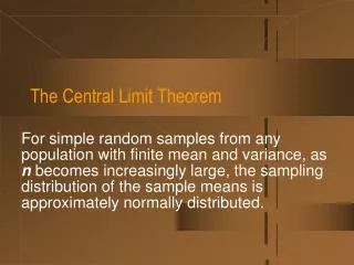
To understand a distribution of sample means, the mean, the standard deviation, and the shape of the distribution all need to be considered. • The Central Limit Theorem* states: For all samples of size n, the sampling distribution of the sample means has a mean equal to the population (theoretical) mean and a standard deviation equal to the standard deviation of the population divided by the square root n: and * Triola, Elementary Statistics
The standard deviation of the simulated sample means has already been calculated. • Using the formula, the standard deviation of the sample means is • This should be compared to the standard deviation of the 201 simulated sample means = – 0.0319
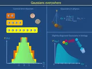
Finally,the shape of the distribution of sample means must be determined. • The mean should be approximately 3.35 • Between three standard deviations less than the mean and three standard deviations greater than the mean should contain about 100% of the scores. • Three standard deviations less than the mean is approximately 3.35 – 3 × 0.3 ≈ 2.4 and three standard deviations greater is approximately 3.35 + 3 × 0.3 ≈ 4.4.
Use this range and a bin size of 0.2 to make a list of values for the Histogram program to sort the sample means into a frequency table. Enter this list somewhere out of the way like cell B32.
To make the frequency distribution, go back to the Histogram program in Data Analysis of the Analysis section in the Data tab and enter: Input Range: G26:GY26 Bin Range: B32:B41 Output Range: D:34 • Again the “Bins” in the distribution table need to be changed to general format in order to make histogram. Change 2.4 to ‘2.4, 2.6 to ‘2.6, and so on.
Select cells D35:E45, click the Insert tab, click Column, and choose the simplest icon in the upper left corner. Put in titles using the Layout tab and ♬♬♬
The third part of the Central Limit Theorem is suggested: For all samples of size n, the sampling distribution of the sample means can be approximated by a normal distribution. Thank you, Dale Nelson, Salt Lake Community College Dale.nelson@slcc.edu http://dknelsonmathteacher.weebly.com Session: S172