Download
1 / 39
390 likes | 409 Views
Explore three scales of cellular system modeling - nanoscale, mesoscale, and macroscale using Molecular Dynamics, Ordinary Differential Equations, and Dynamic Cellular Automata for accurate simulations. Understand the challenges and benefits of each scale in simulating complex biological processes.

E N D
AGENTS BASED MODELLING AND SIMULATION OF CELLULAR PROCESSES
Cellular systems and subsystems can be simulated at three different scales:
Nanoscale (10-10 10-9) At the level of atoms and molecules (nanoscale) we typically use molecular dynamics (MD) or Brownian dynamics to model the behavior of 100’s to 1000’s of discrete atoms over relatively short periods of time (10-10 to 10-9 s) and space (10-9 m). MD is Fully deterministic Used to simulate state or conformational changes, predict binding affinities, investigate single molecule trajectories and model stochastic or diffusive interactions between small numbers (<5) of macromolecules it is still impossible to model large numbers of molecules (>106) or macromolecules (>102) over extended periods of times and space (milliseconds to millimetres).
Macroscale (10-3) On the other side of the spectrum there are the continuum approaches Molecules essentially lose their discreteness and become infinitely small and infinitely numerous To model at the macroscale or continuum level, we must turn to ordinary (ODE’s) or partial differential equations (PDE’s) to describe our systems of interest. Time dependent ODE’s are routinely used to describe individual enzyme reactions, diffusion events and other rate-dependent processes Most of the nowadays systems biology is based on Differential Equations
Not all systems are amenable to descriptions by differential equations. For instance, state changes, discontinuities, irregular geometries or discreteness (low copy numbers) are not easily described by differential equations. Furthermore, due to their continuum nature, the solutions to differential equations always generate smooth curves or surfaces that fail to capture the true granularity or stochasticity of living systems. An additional challenge to using differential equations is that they require a strong foundation in mathematics, a detailed knowledge of many (sometimes unknowable) rate constants or initial conditions, and a powerful “solver” to generate solutions.
Mesoscale (10-8 10-7) Macromolecules can still be treated as discrete objects occupying a defined space or volume. Mesoscale models display the stochasticity or granularity found in real biological systems. Because Brownian motion dominates over all other forces at this scale, it turns out that significant dynamic simplifications are possible with mesoscale modeling. These simplifications potentially allow very long time scales and large numbers of entities or reactions to be modeled
Dynamic Cellular Automata (“agent based modeling”) Simulated Brownian motion on a 2D grid Simple pairwise interaction rules . DCA can be used to easily and accurately model a variety of spatial and temporal phenomena including: macromolecular diffusion, viscous drag, enzyme rate processes, the Kreb’s cycle, and complex genetic circuits.
Cellular Automata Cellular automata (CA) are mutli-object computer simulation tools that consist of large numbers of simple identical components with local interactions layered over a lattice or grid. The states or values of the components evolve synchronously in discrete time steps according to identical rules. The value of a particular site is determined by the previous values or states of a neighbourhood of sites around it. Originally conceived by von Neumann in the late 1940’s cellular automata have been used to model a wide range of physical processes including heat flow, spin networks and reaction-diffusion processes Cellular automata also have a long history in biological modeling. Indeed, one of the first computer applications in biology was a CA simulation called Conway’s Game of Life [Gardner, 1970]. This simple model simulated the birth, death and interaction between cells randomly scattered over a square lattice or grid. The fate of every cell was determined according to three pair-wise interaction rules. These interaction rules were typically "if-then-else" statements describing what a cell could do depending on the number of adjacent neighbors. Nowadays, perhaps the most widespread and familiar use of CA can be found in popular computer games such as SimCity, SimEarth and The Sims
Macromolecules at the mesoscale appear as discrete, but largely unstructured tubes, cubes or spheres. • The objects (proteins, DNA) can still interact with each other, but their interactions are no longer constrained or described by shape complementarity or lock-and-key fitting as they would be if we were modeling at the nanoscale. • Instead the interactions can be described by simple, logical operations or statements such as: • If A is adjacent to B, then A binds B. • While C is bound to D, produce F. • If A is adjacent to M, then M is converted to P • DCA differs from conventional CA in that the DCA model attempts to simulate real motions via Brownian dynamics.
SimCell A very general structure that would allow the accurate simulation of most cellular pheonomena (transport, enzyme kinetics, metabolism, reaction-diffusion, signaling, genetic circuits and transcription/translation) 4 kinds of component molecules: 1) small molecules (metabolites, ligands), 2) membrane proteins (which can only exist in membranes), 3) soluble protein/RNA molecules and, 4) DNA molecules (which are non-mobile). Because cells are composed of subcellular organelles and because some simulations require compartmentalization of reactants, products or metabolites, we also introduced a fifth type of molecule or super-molecule: 5) the membrane (non-mobile entities that describe boxes or borders that may be permeable or impermeable to certain molecules )
3 major types of pairwise interactions: 1) bind and stick (B&S) , 2) touch and go (T&G) , 3) directional transport (TR) . Molecules that bind and stick have association and dissociation constants or on/off probabilities and rates. Many protein receptors, DNA binding proteins, catabolic repressors and gene activators will bind and stick to a target molecule. Under the SimCell rules, molecules that bind and stick with each other must necessarily transform themselves into a new entity (a third molecule) or, in the case of DNA binding, lead to changes in the creation or transcription rate of a third molecule. Non-interacting molecules will typically touch and go (bump), always leaving each other in tact. However, some touch and go operations do lead to a molecular transformation, particularly when we consider enzymes such as metabolic enzymes, nucleases or proteases. While enzymatic catalysis technically involves some binding, given the time step used in our mesoscale simulations (1 ms), catalysis is, for all intents and purposes, instantaneous. In these enzymatic touch and go operations, two objects will meet leaving one object in tact and one transformed. Finally, in transport operations an object (usually a small molecule) is taken and almost instantaneously (< 1 microsecond) moved across a barrier (usually a membrane)
In SimCell the motion for all objects (except membranes and DNA molecules) is performed in a step-wise fashion over the space defined by a regular 2-dimensional grid. Within the grid each object or molecule occupies a square, typically measuring 3 nm on a side. The choice of 3 nm as the standard grid increment is based on a number of criteria. The diameter for an average protein is approximately 3 nm, The average width of a cellular membrane is approximately 3 nm, The average width of a supercoiled DNA molecule is about 3 nm The average velocity of a macromolecule in a cell is approximately 3 nm per millisecond This macromolecular diffusion rate also helps to define a time step that is appropriate for these mesoscale simulations – namely a millisecond.
Macromolecules such as proteins or RNA molecules are allowed to occupy only a single square at a time, whereas up to 100 small molecules (which typically measure 0.3 nm across) are permitted to occupy a single square. This multiple occupancy rule for small molecules avoids the need to reduce the grid size and time steps by a factor of 10. This simplification also makes the simulations run much faster. Small molecules are known to diffuse at approximately 50 nm/ms, or approximately 10 times faster than macromolecules. To accommodate their faster diffusion rate, SimCell performs 10 small molecule movements/interaction checks for each macromolecular movement step.
Validations -Enzyme kinetics -Macromolecular diffusion -Metabolic simulation -The repressilator gene circuit
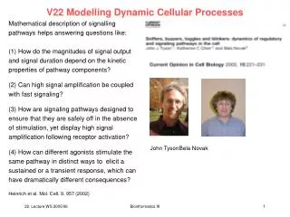
Formal computational modelling approach to model a crucial biological system—the intracellular NF-kB signalling pathway. The pathway is vital to immune response regulation, and is fundamental to basic survival in a range of species. Alterations in pathway regulation underlie many diseases, including atherosclerosis and arthritis. Modelling of individual molecules, receptors and genes provides a more comprehensive outline of regulatory network mechanisms than previously possible with equation-based approaches.
Activation of the NF-kB pathway is controlled by inhibitors of NF-kB (IkB) proteins, which sequester the majority of NF-kB in the cytoplasm as complexes by masking their nuclear localisation signals. During activation, IkB is phosphorylated by IkB kinases (IKK), causing its destruction. The newly freed NF-kB is consequently transported into the nucleus, inducing inflammatory genes, including those encoding IkB, thus regulating the pathway through negative feedback
Due to the complexity of signalling pathways, large numbers of linked ODEs are often necessary for a reaction kinetics model. (ODEs) to describe each chemical concentration with time. This implicitly assumes homogeneity, treating the cell as a well-mixed bag of chemicals. Such models can be narrowly limited in the range in which they function properly, which is at odds with the robustness of nature. The many interdependent differential equations can be very sensitive to their initial conditions and constants, with small changes in these sometimes causing huge behavioural changes in the system. Solutions may be liable to describe unrealistic or impossible behaviour, such as negative concentrations, unless the initial conditions and constants are correct to a high degree of precision. While differential equation models may produce useful results under certain conditions, they provide a rather incomplete view of what is actually happening in the Cell Spatial effects on pathways are also often crucial, but again difficult to incorporate into such a model, though partial differential equations (PDEs) could theoretically be used.
Many aspects of life involve the interaction of multiple components and subunits and the corresponding emergence of both form and function. Agent-based (sometimes called individual based) approaches – whereby the components are represented as autonomous software artefacts that exist within a software environment – provide a mechanism for understanding their behaviour through simulation of the actual behaviour of the equivalent biological system.
Communicating X-machine Various computational models exist to represent agents, though the Communicating X-machine is perhaps the most powerful and intuitive (Eleftherakis et al., 2001; Balanescu et al., 1999). Agent-based modelling has recently been applied to a variety of biological systems, including insect communities and epithelial tissue (Jackson et al., 2004a, 2004b; Walker et al., 2004; Holcombe et al., 2003).
An agent-based chemical model does not have the same restrictions as a differential equation model Any number (low or high, within computational limitations) and distribution of molecules can be modelled, spatial concerns can easily be accounted for, as can time delays. An agent-based model also provides a clearer picture of what is actually occurring in the cell. More details must be defined. The movement of agents must be explicitly stated. Agents must at least move around enough to regularly collide. It is vital that the agent-based model is able to deal with individual interactions of molecule agents with the same accuracy as reaction kinetics.
Developing software for agent-based systems can make use of many modern software engineering techniques, including decomposition, or dividing a problem into small, manageable parts, abstraction, or choosing which details of a problem to model and which to suppress, and organization, or identifying and managing the relationships among the various system components. The agent-based model is a bottom-up paradigm wherein the lowest level entities, called agents, interact with each other autonomously. An agent is an encapsulated computer system that is situated in some environment and that is capable of flexible, autonomous action in that environment in order to meet its design objectives
The agents are situated in space and time and have some properties and certain sets of local interaction rules. Though intelligent, they cannot by themselves deduce the global behavior resulting from their dynamic interactions. The system evolves from the micro level to the macro level. Thus agent-based modeling uses a bottom-up design strategy rather than a top-down strategy. Agents are commonly assumed to have well-defined bounds and interfaces, as well as spatial and temporal properties, including such dynamic properties as movement, velocity, acceleration, and collision. They exist in an environment which they sense and can communicate with through their interfaces. They are assumed to respond in a timely manner to changes in their environment. They are autonomous, encapsulating a state and changing state based on their current state and information they receive.
ODE method does not account for spatial aspects. Dimerization of monomer proteins, dissociation of dimers, Repressor binding to Operator regions, and RNA Polymerase binding to Promoter regions are all processes in which the spatial aspects play a crucial role. Agent-based models account for these spatial and temporal aspects and hence can be closer to actual biological processes. The greater the number of details that go into describing the behavior of the system, the greater is the computational power that is required to simulate the behaviors of all constituent agents. This is a limitation in modeling large systems using ABM. A reasonable approach is to provide several levels of abstraction and granularity, which can be chosen depending on the level of detail needed and the computational resources available. Here we are modeling reactions at the molecular level, for a relatively small number of molecules, so we have chosen a very fine-grained level of modeling.
Agents simulators There are a few popular packages for simulation of decentralized systems which provide 2D visualization. MASON Repast Swarm StarLogo
BREVE BREVE is a 3D simulation engine developed to provide quick and easy simulations of decentralized systems. It is an open-source package available for Mac OS, Linux, and Windows platforms. It allows users to define and visualize decentralized agent behaviors in continuous time and continuous 3D space. The package comes with its own interpreted object-oriented scripting language called steve, an OpenGL display engine, and collision detection. BREVE also has a library of built-in classes and provides graphical 3D visualization and collisions between 3D bodies. These features remove a significant amount of programming overhead.
LAMBDA PHAGE – E. coli Escherichia coli (E. coli) is an intestinal bacterium and is a commonly studied prototype for bacteria. When a passively infected E. coli bacterium is exposed to a dose of ultraviolet light, it stops reproducing and starts to produce a crop of viruses called phage lambda into the culture medium. This process of rapid reproduction of the phage lambda viruses is called lysis. The newly-formed lambda phages multiply by infecting fresh bacteria. Some of the infected bacteria lyse further, causing more phages to be produced, whereas some bacteria may carry the phage in a passive form, causing the bacteria to grow and divide normally. This process of passive reproduction of the phage lambda is called lysogeny