Download
1 / 20
200 likes | 313 Views
This document explores the essential aspects of estimating available bandwidth (Avail-Bw) for transport layer protocols (TLP). It covers current estimation techniques, requirements for effective TLP estimation, and presents a proposed solution to enhance estimation accuracy and practicality. Key concepts include the definition of available bandwidth, utilization of links at specific time intervals, and the importance of selecting appropriate congestion window sizes to optimize TCP throughput. Open questions surrounding utilization and bandwidth estimation are also discussed.

E N D
Estimating Available Bandwidth for a Transport Layer Protocol Cesar D. Guerrero
Outline • Background • Avail-Bw for a TLP? • Current Avail-Bw Estimation Approaches • TLP Estimation Requirements • Proposed solution? • Open questions
Utilization 1 0 t Utilization of a link • The utilization of a link in a specific instant of time tcan be only either 0 (if the link is idle) or 1 (transmitting a packet at full link capacity) • The average utilization of a link iduring the time interval (t, t+τ ) is: • In the example, the link is used 15 out of 30 time intervals. So, the average utilization is 0.5.
t A(t) t Available Bandwidth • The Available Bandwidth is the unutilized capacity of the link during a period of time. • The Available Bandwidth of a link iduring the time interval (t, t+τ ) is: • The available bandwidth of the end-to-end path is:
t t t t t t . . . A(t) 3 1 2 5 . . . ksamples 4 t Available Bandwidth (cont) • A(t) is a stationary random process at least over short intervals of time. • The longer τ and k, the more accurate (But the more intrusive and slow)
Narrow link Tight link Capacity and Available Bandwidth The link with the minimum transmission rate determines the capacity of the path (narrow link) while the link with the minimum non-utilized capacity (tight link) limits the available bandwidth.
Outline • Background • Avail-Bw for a TLP? • Current Avail-Bw Estimation Approaches • TLP Estimation Requirements • Proposed solution? • Open questions
Why Avail-Bw for a TLP? • To increase TCP throughput by selecting a CongWin size according to the available bandwidth in the end to end path TCP Throughput = CongWin/RTT [bytes/sec] • The maximum TCP buffer size in many UNIX-based OS is 256 KB. That is, for an RTT of 150 ms, the maximum throughput will be no more than 15 Mbps. For a 40 ms link, no more than 50 Mbps.
Outline • Background • Avail-Bw for a TLP? • Current Avail-Bw Estimation Approaches • TLP Estimation Requirements • Proposed solution? • Open questions
Δout P2 P1 Δin Probing traffic at rate Ri Packet length: L Δout P2 P1 P2 P1 Cross traffic at rate Rc Tight link capacity: Ct Ri A Ri > A Basic Model: Single link with fluid traffic During Δin = L / Ri Total amount of traffic arriving = Xc + L = (Δin Rc)+ L Maximum amount of traffic can be transmitted = Δin Ct Queue increasing = Δq = Δin (Ri – A) OWD increasing = Δd = Δq / Ct Output interarrival =Δout =Δin + Δd Queue increasing = Δq = 0 OWD increasing = Δd = 0 Output interarrival =Δout =Δin
Probing packets delay increases when the probing rate is higher than the available bandwidth in the path. • Sender transmits a periodic probing stream with rate Ri(n) • Receiver measures output rate Ro(n) and determines if Ri(n) > A to notify the sender about the next Ri(n+1) • The objective is to find the point when the delays start to increase. IGI Delphy Spruce Pathload. TOPP Pathchirp PTR Current approaches: Probe Gap Model Probe Rate Model • Measure the packet pair dispersion. • That dispersion has a relation with the cross traffic rate at the tight link. • Assumption: the tight link capacity is known and Ri>A • Available bandwidth:
Outline • Background • Avail-Bw for a TLP? • Current Avail-Bw Estimation Approaches • TLP Estimation Requirements • Proposed solution? • Open questions
TLP estimation requirements • Zero overhead • Convergence time according to the congestion events distribution • “Acceptable” accuracy
Outline • Background • Avail-Bw for a TLP? • Current Avail-Bw Estimation Approaches • TLP Estimation Requirements • Proposed solution? • Open questions
In the gray region, the tool reports the available bandwidth Figure copied from the paper “Pathload: A Measurement Tool for End-to-end Available Bandwidth” by M. Jain and C. Dovrolis Estimation Approach:Probe Rate Model • Pathload is the most accurate and stable tool Figure copied from the paper “Experimental and Analytical Evaluation of Available Bandwidth Estimation Tools” by Cesar D. Guerrero and Miguel A. Labrador. • It sends a fleet of probing streams to fill the available bandwidth. • The one-way delay increases when the rate of the probing traffic is higher that the available bandwidth.
ip_output() ip_input() Zero overhead solution:TCP with Inline Measurement (ImTCP) Application Programs Socket interface TCP Layer tcp_output() tcp_input() Data packets ACK packets ImTCP buffer Measurement Program IP Layer Network Interface Figure based on the paper “Implementation and evaluation of an inline network measurement algorithm and its application to TCP-based service” by T. Tsugawa, G. Hasegawa, and M. Murata
ε Ri Whereεis called inter-packet strain: Now we have a first-order polynomial model in Rigiven by: Available Bandwidth Real-Time solution:Kalman Filters (Model) Based on the paper “Real-Time Measurements of End-to-End Available Bandwidth using Kalman Filtering” by S. Ekelin, M. Nilsson, E. Hartikainen, A. Johnsson, JE. Mangs, B. Melander, and M. Bjorkman
The available bandwidth is described by the state vector where, Real-Time solution:Kalman Filters (Implementation) We want to know x, but we only are able to observe εwhich is affected byRi The available bandwidth is affected by noise w, and the measurements of εby a noisev The filter takes Ri(k), ε(k) and an estimate x(k) as inputs, and computes a new estimate x(k+1) Based on the paper “Real-Time Measurements of End-to-End Available Bandwidth using Kalman Filtering” by S. Ekelin, M. Nilsson, E. Hartikainen, A. Johnsson, JE. Mangs, B. Melander, and M. Bjorkman
Outline • Background • Avail-Bw for a TLP? • Current Avail-Bw Estimation Approaches • TLP Estimation Requirements • Proposed solution? • Open questions
Open questions • How often available bandwidth estimation is required? • ImTCP obtain it every 1 to 4 RTTs • How is computational performance affected when TCP buffer size is increased? • Extended Kalman Filter? Particle filters?