Ray-tracing
Ray-tracing. Photorealism Reflection, Refraction Bump maps. Overview. Textures review Lighting re-visited Photorealism + Global Illumination Reflection Refraction Bump Maps / Normal maps Lab. © Gilles Tran . The Phong Illumination algorithm cannot generate images like these.

Ray-tracing
E N D
Presentation Transcript
Ray-tracing Photorealism Reflection, Refraction Bump maps
Overview • Textures review • Lighting re-visited • Photorealism + Global Illumination • Reflection • Refraction • Bump Maps / Normal maps • Lab
The Phong Illumination algorithm cannot generate images like these
The Rendering Equation 0 if x and x’ are not mutually visible 1/r2where • I(x, x’) = intensity of light passing from x to x’ • (two point transport) • g(x, x’) = • (geometry factor) • e(x, x’) = intensity of light emitted by x and passing to x’ • ρ (x, x’, x”) = bi-directional reflectance scaling factor for light passing from x” to x by reflecting off x’ • S = all surfaces in the scene A physicists representation of light transport in the scene, describing the amount of light going from any point x to another point x’: [Kajiya 1986] Attenuation (distance from x to x’)
Light_transport_from B to A: Emmitance of B Visibility of B from A Distance to B from A Also: Reflectance of B Light_transport_from Ci to B Emmitance of C Visibility of C from B Distance to C from B A B C2 C1 C3 D1
Assumptions • I on both sides of the equation suggests an infinitely recursive path of light transfer. • We need to make some simplifying assumptions in order to solve this equation • Local Illumination algorithms assume light only “bounces” once travelling from light source to a point in the scene and then to the eye • Global Illumination algorithms account for light transport between several points on the scene before reaching the eye (several bounces) • Thus can account for refraction, shadows, reflections etc. Less realistic, usually used in real-time rendering More expensive, usually used in off-line rendering
Local vs. Global Illumination Global Local Illumination at a point can depend on any other point in the scene Illumination depends on local object & light sources only
A photo-realistic rendering algorithm Current ray tracing methods are attributed to Turner Whitted (Bell Labs. 1980) Whitted Illumination Model First implementation of ray tracing in computer graphics = Appel (IBM 1968) Recursive Raytracing, 1979 Recorded in “An Improved Illumination Model for Shaded Display” (Bell Labs, 1980). Ray Tracing
Albrecht Dürer (1471-1528) Ray-tracing based on ideas employed since early Renaissance artists e.g. daVinci & Dürer
Ray Tracing • The Direct Diffuse Term Ilocal is calculated empirically (using Phong illumination) • In the global ray-traced terms, diffusion of light due to surface imperfections is totally ignored. I(P) = Ilocal(P) + krgI(Pr) + ktgI(Pt) Local term (as in Phong) Reflected Transmitted
Ray Tracing from Eye Tracing from light source Traditional ray-tracing Starting at the light position traces many rays that never reach the eye. Thus the traditional ray-tracing method is to start at the eye and trace rays back-wards to the source.
Eye Ray and Object Intersection Cast a ray from camera position through each pixel into the scene. Calculate where this intersects with objects in the scene. Get the first intersection.
Diffuse Term • Extend a “Shadow Feeler” (or light ray) and see if it is occluded by an object in the scene • If so the object is in shadow from this light source • Otherwise solve the phong model to calculate the contribution of this point to the colour of the pixel. • If object is diffuse stop here.
Reflection • For this new ray, we will again check whether… • it intersects an object, • if so is this object in shadow • what is the contribution of this object to the colour of the pixel? • Each ray contributes to the colour of the pixel it originated from • If object is specular THEN create a ray in the direction of perfect specular reflection.
Similarly if the object is transmissive (not-opaque) then generate a transmitted (or refracted) ray and repeat… Refraction
The Angle of Refraction Air Air Air Glass Diamond Water • When light passes from a material of one optical density to another it changes direction. • The amount by which the direction changes is determined by the optical densities of the two media. • Optical density (and thus the amount of bending is related to a value we call the refractive index of the material.
Material Index of Refraction Index of Refraction (ior) Vacuum 1.0000 <--lowest optical density Air 1.0003 Ice 1.31 Water 1.333 Ethyl Alcohol 1.36 Plexiglas 1.51 Crown Glass 1.52 Light Flint Glass 1.58 Dense Flint Glass 1.66 Zircon 1.923 Diamond 2.417 Rutile 2.907 Gallium phosphide 3.50 <--highest optical density You can try these refracted index values in POVRay.
Ray Tracing Issues • Cast a ray • Determine Intersections • For closest Intersection: • Extend light(shadow feeler) ray + calculate local term • Spawn Transmitted Ray (step 1) • Spawn Reflected Ray (step 1) I(P) = Ilocal(P) + krgI(Pr) + ktgI(Pt)
Ray Tree The spawning of reflected and refracted rays can be represented in tree structure.
Terminating Recursion • All of the spawned rays contribute to the pixel that the tree originated from. • However each new ray contributes less and less to the pixel. • Unlike in the real-world, we can’t keep bouncing around for ever so we stop the recursion at some stage recursion clipping. • Stop after a set number of bounces. • Or stop when the contribution becomes less than a certain value.
Recursion Clipping max level = 1 max level = 2 Very high maximum recursion level max level = 3 max level = 4
Object Intersection • Intersection testing is solved mathematically. But is an inherently expensive geometrical problem. (out of the scope of current lecture) Where does ray intersect object? Where does ray intersect scene?
The Ray Tracing Algorithm Intersection trace(ray, objects) { for each object in scene intersect(ray, object) sort intersections return closest intersection } for each pixel in viewport { determine eye ray for pixel intersection = trace(ray, objects) colour = shade(ray, intersection) }
The Ray Tracing Algorithm colour shade(ray, intersection) { if no intersection return background colour for each light source if(visible) colour += Phong contribution if(recursion level < maxlevel) { ray = reflected ray intersection = trace(ray, objects) colour += refl*shade(ray, intersection) ray = transmitted ray intersection = trace(ray, objects) colour += trans*shade(ray, intersection) } return colour }
Reflection finish { reflection 0.5 //phong etc… }
Translucency texture { pigment { rgbf <1, 1, 1, .8> } } Filter value of 0 is fully opaque, 1 is fully transparent.
Refraction texture { pigment { rgbf <1, 1, 1, .8> } } interior { ior 3 }
Caustics texture { pigment { rgbf <1, 1, 1, .8> } } interior { ior 3 caustics 1 }
Bump Mapping A “real” bump distorts the directions of the normals (this effects calculations of light reflectance) “Fake” bumps created by distorting the normals although the geometry is still flat. A bump-map texture applied to a flat polygon.
Normal Maps • We can add bumps, dents, wrinkles, ripples and waves to our objects. box { < -4, -.25, -4 > < 4, .25, 4 > pigment { White } finish { reflection .4 } normal { //add normal pattern here **** } } Sample Scene (no normal maps)
Bumps normal { bumps 1 }
Dents normal { dents 1 }
Wrinkles normal { wrinkles 1 }
Ripples normal { ripples 1 }
Waves normal { waves 1 }
Bump Map normal { bump_map { gif "bumpmap.gif" } rotate 90*<1, 0, 0> scale 8 }
Lab • Reflection in POV-Ray: use the reflection parameter in the finish statement to generate photorealistic reflective surfaces • Refraction in POV-Ray: use the interior definition and ior values to generate photorealistic refraction • Use a bump map/ normal map to generate some of the following effects:
Normal Maps ripples bumps dents wrinkles
Bump Map Bump Map image file https://www.cs.tcd.ie/John.Dingliana/bumpmap.gif (or use your own)
POV-Ray Objects • If you want to create more interesting scenes with real world objects, you can find POV-Ray objects on several sites including: • http://objects.povworld.org/cat/