Markowitz Mean-variance
Markowitz Mean-variance. Sequence Of MPT Material. Basic Return vs Risk Optimizing the Risky Portfolio Risk Aversion / Utility Function Allocate Between Risk-free asset and Risky Asset (CAL). Stocks vs Bonds Markowitz Mean-Variance Asset Allocation. Going In Reverse: the CAPM.


Markowitz Mean-variance
E N D
Presentation Transcript
Sequence Of MPT Material • Basic Return vs Risk • Optimizing the Risky Portfolio • Risk Aversion / Utility Function • Allocate Between Risk-free asset and Risky Asset (CAL) • Stocks vs Bonds • Markowitz Mean-Variance Asset Allocation • Going In Reverse: the CAPM Calculates theoretical expected return for individual assets based upon covariance with “the market” and the risk-free return.
Evolution of Variance Measures in Studying MPT Individual Assets/Asset Class Variance (Return for Period – Mean Return) ^2 Paired Covariances (Asset 1 Return – Mean) x (Asset 2 Return – Mean) Portfolio Variance For 2 assets: Asset 1 Variance + Asset 2 Variance + 2 x Weighted Covariance
Background Assumptions • As an investor you want to maximize the returns for a given level of risk. • Your portfolio includes all of your assets, not just financial assets • The relationship between the returns for assets in the portfolio is important. • A good portfolio is not simply a collection of individually good investments.
Markowitz Portfolio Theory • Derives the expected rate of return for a portfolio of assets and an expected risk measure • Markowitz demonstrated that the variance of the rate of return is a meaningful measure of portfolio risk under reasonable assumptions • The portfolio variance formula shows how to effectively diversify a portfolio
Markowitz Portfolio Theory Assumptions • Investors consider each investment alternative as being presented by a probability distribution of expected returns over some holding period. • Investors maximize one-period expected utility, and their utility curves demonstrate diminishing marginal utility of wealth. • Investors estimate the risk of the portfolio on the basis of the variability of expected returns.
Markowitz Portfolio Theory Assumptions • Investors base decisions solely on expected return and risk, so their utility curves are a function of expected return and the expected variance (or standard deviation) of returns only. • For a given risk level, investors prefer higher returns to lower returns. Similarly, for a given level of expected returns, investors prefer less risk to more risk.
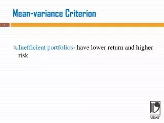
Markowitz Portfolio Theory • Under these five assumptions, a single asset or portfolio of assets is efficient if no other asset or portfolio of assets offers higher expected return with the same (or lower) risk, or lower risk with the same (or higher) expected return.
Alternative Measures of Risk • Variance or standard deviation of expected return (main focus) • Based on deviations from the mean return • Larger values indicate greater risk • Other measures • Range of returns • Returns below expectations • Semivariance – measures deviations only below the mean
Characteristics of Probability Distributions 1)Mean: most likely value 2) Variance or standard deviation 3) Skewness * If a distribution is approximately normal, the distribution is described by characteristics 1 and 2.
Single Factor Mean-Variance Model • Expected Return • Expected Variance
Portfolio Standard Deviation Calculation • The portfolio standard deviation is a function of: • The variances of the individual assets that make up the portfolio • The covariances between all of the assets in the portfolio • The larger the portfolio, the more the impact of covariance and the lower the impact of the individual security variance
Constructing Risky Portfolios • E(rp) still as easy as ever –simple weighted average of asset E(r)s • Variance of the risky portfolios for two assets = • σp2 = wA12 x σA12 +wA22xσA22 + 2 x wA1 x wA2 x COVAR(A1,A2) • Another case of the general formula presented as a special case (It’s a global conspiracy) • The general rule is just to take the weighted average of all of the covariances for all possible paired sets in the portfolio
Generalize The Portfolio Variance Calculation σp2 = wA12 x σA12 +wA22xσA22 + 2 x wA1 x wA2 x COVAR(A1,A2) Now with the general rule: σp2 = wA1 x wA1x Covar (A1,A1) + wA2 x wA2 x Covar (A2,A2) + wA1 x wA2 x Covar (A1,A2) + wA1 x wA2 x Covar (A1,A2) • Covar(A1,A1) =σA12 • Note that there are now 4 terms (2 x 2) for 2 assets
The General Formula Is Easier To Use In A Worksheet Environment • We use a covariance matrix Note that this looks just like the Mean-Variance Worksheet • Then we need to weight each covariance term • for the asset weighting in the portfolio
Adding Asset Weights • Here is a “bordered” covariance matrix for a portfolio with 60% asset 1 and 40% asset 2 – the asset weights are the borders Note that this matrix is also on the Mean-Variance Worksheet
One Final HintRevisiting Covariance vs Correlation Coefficient • The formula to calculate ρ ρ1,2 = Covar (A1,A2) / σA1 x σA2 • If we know ρ1,2 and need to calculate Covar(A1,A2) : Covar (A1,A2) = ρA1,A2 x σA1 x σA2 This formula is used in B6 to C12 and B16 to H22 to calculate the covariance matrix. B16 to H22 should look familiar.
Diversification And Hedging Diversification Hedging 1.0 0.0 -1.0 Correlation Coefficient
Implications for Portfolio Formation • Assets differ in terms of expected rates of return, standard deviations, and correlations with one another • While portfolios give average returns, they give lower risk • Diversification works! • Even for assets that are positively correlated, the portfolio standard deviation tends to fall as assets are added to the portfolio
Implications for Portfolio Formation • Combining assets together with low correlations reduces portfolio risk more • The lower the correlation, the lower the portfolio standard deviation • Negative correlation reduces portfolio risk greatly • Combining two assets with perfect negative correlation reduces the portfolio standard deviation to nearly zero
The Efficient Frontier • The efficient frontier represents that set of portfolios with the maximum rate of return for every given level of risk, or the minimum risk for every level of return • Frontier will be portfolios of investments rather than individual securities • Exceptions being the asset with the highest return and the asset with the lowest risk (This is true for Minimum Variance Frontier, not the Efficient Frontier)
Efficient Frontier B E(R) A Standard Deviation of Portfolio Return Efficient Frontier and Alternative Portfolios C
The Efficient Frontier and Portfolio Selection • Any portfolio that plots “inside” the efficient frontier (such as point C) is dominated by other portfolios • For example, Portfolio A gives the same expected return with lower risk, and Portfolio B gives greater expected return with the same risk • Would we expect all investors to choose the same efficient portfolio? • No, individual choices would depend on relative appetites return as opposed to risk
Unsystematic (diversifiable) Risk Total Risk Standard Deviation of the Market Portfolio (systematic risk) Systematic Risk Number of Stocks in the Portfolio The Portfolio Standard Deviation
Optimization • What is it? • What do we optimize? • The efficient frontier is a series of portfolios optimized (lowest variance) for a series of possible E(r)s • We graph some sub-optimal portfolios • (below the “kink”) • The endpoints are the lowest and highest E(r) assets includable in the portfolio
The Two-Asset Example • Easiest to graph and comprehend • Easy to optimize (formula-based) • The graph line is set up by taking evenly-spaced mixes of two assets • Low end of the graph is 100% the smaller E(r) asset, top end is 100% the larger E(r) • Graph is same style as our Utility graph
The Efficient Frontier and Investor Utility • An individual investor’s utility curve specifies the trade-offs she is willing to make between expected return and risk • Each utility curve represent equal utility; curves higher and to the left represent greater utility (more return with lower risk) • The interaction of the individual’s utility and the efficient frontier should jointly determine portfolio selection
The Efficient Frontier and Investor Utility • The optimal portfolio has the highest utility for a given investor • It lies at the point of tangency between the efficient frontier and the utility curve with the highest possible utility
U3’ U2’ U1’ Y U3 X U2 U1 Selecting an Optimal Risky Portfolio
Utility / Risk Aversion Utility = E(r new asset) - .005 x Aversion x σ2(new asset) U = E(r new asset) - .005 x A x σ2(new asset) If Utility > Risk Free Return, Asset Fits Within Your Risk Profile
Utility Calculations For a Risk Aversion Level of 4: Risk-Free Rate = 5.00 Vanguard S&P 500 (VFINX): U = 11.24 - .005 x 4 x 430.13 = 2.64 Fidelity Japan (FJPNX): U = 8.21 - .005 x 4 x 2660.23 = -45.00
Utility Curve Graph line represents the portfolios with utility equal to sample Port Risk aversion level (A) is constant
Investor Differences and Portfolio Selection • A relatively more conservative investor would perhaps choose Portfolio X • On the efficient frontier and on the highest attainable utility curve • A relatively more aggressive investor would perhaps choose Portfolio Y • On the efficient frontier and on the highest attainable utility curve
Risky Assets Versus The Risk-free Asset An Example: Risk-free rate = 4% Risky Assets/Portfolio E (r) = 9% Risky Assets/Portfolio σ = 8% What is the risk premium?
The Risk-Free Asset Is Not Included When Calculating Optimal Risky Portfolios • Because σ = 0, there is no diversification benefit • Therefore, adding the risk-free asset cannot improve the efficient frontier • The risk-free asset plays a critical role AFTER the optimal risky portfolios and efficient frontier have been determined • Utility can be improved with the subsequent addition of the risk-free asset
Risky Assets Versus the Risk-free AssetCombinations With No Borrowing RiskyPortfolio 9% E (r) 4% σ 0 8%
Risky Assets Versus the Risk-free AssetCombinations With Borrowing at R(f) RiskyPortfolio 9% E (r) 4% σ 0 8%
Risky Assets Versus the Risk-free AssetCombinations With Borrowing at R(f) RiskyPortfolio 9% E (r) 4% y < 1 y > 1 σ 0 8%
Risky Assets Versus the Risk-free AssetCombinations With Borrowing at R(f) + 1% RiskyPortfolio 9% E (r) 4% y < 1 y > 1 σ 0 8%
Risky Assets Versus the Risk-free AssetCombinations With Borrowing at R(f) + 1% RiskyPortfolio 9% This is the Capital Allocation Line CAL E (r) 4% y < 1 y > 1 σ 0 8%
Risky Assets Versus the Risk-free AssetCombinations With Borrowing at R(f) + 1% RiskyPortfolio 9% You can solve for utility curves that will intersect the CAL at the optimal point Y=(Erp-rf)/(.01xAxVp) E (r) 4% y < 1 y > 1 σ 0 8%
Annualization of Variance / S.D. Quarterly Annual σq2 = .36 x 4 1.44 σq = .60 x SQRT(4) 1.20 Note: 4=periods / year Monthly Annual σm2 = .12 x 12 1.44 σm = .3464 x SQRT(12) 1.20