Download
1 / 31
310 likes | 372 Views
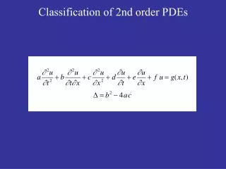
This research explores the generation of structured grids using elliptic partial differential equations transformation. The main aim is to construct a uniform grid within the computational domain by solving boundary-value problems. Techniques for structured grid generation, curvilinear coordinates, and metric tensor are discussed. Challenges and advantages of utilizing curvilinear coordinates are addressed, highlighting the importance of maintaining grid quality in regions with high flow gradients. The transformation of physical boundaries to curvilinear coordinates aids in efficient calculations within the computational domain. The structured grid system enforces restrictions on grid connectivity, ensuring smooth and orthogonal distribution while solving complex systems of equations. The study emphasizes the importance of preserving the grid structure for accurate solutions and efficient numerical methods.

E N D
Generation of Structured Grid by Solving Elliptic PDEs Dzhmova Olga
The main problem • For generation of structured grid we use the transformation of coordinates • The main aim of this transformation is the construction of uniform grid at the computational domain where physical boundaries fit (lie in) the coordinate system
Abstract • Curvilinear coordinates • Transformation of coordinates • Metric tensor • Generation of structured grid • Classification of techniques for structured grid • Elliptic grid generation • Conclusion
Curvilinear coordinates • the object in the physical domain is transposed to the rectangular in the curvilinear coordinates • it is efficient to do calculations at the computational domain
Curvilinear coordinates(an example) At the physical domain the point with coordinates correspond to the point (j,k)
Curvilinear coordinates The mapping of the physical domain to the domain of curvilinear coordinates can do the concentrate of coordinate lines in the areas of the physical domain where expected appearance of large gradients. If the areas of large gradients are changed with time, for e.g. moving of air-blast, the physical grid can be reformed so, that the local grid will be so fine for getting the solution with required precision.
Curvilinear coordinates • There are some difficulties when we use the curvilinear coordinates. • to define the form of equations in the curvilinear coordinates • at this questions there are some additional terms (parameters of transformation, for e.g. ) which are additional source of errors
Transformation of coordinates Assume, that a one-to-one mapping can be established between physical and curvilinear coordinates, which can be written as: and correspondingly Using these functional dependences the equations can be transform to the form, which contain partial derivations over
Transformation of coordinates As an example, the first-order derivatives u, v, and w over x, y, z. ,where (1.1) J – the matrix transformation of Jacobi.
Transformation of coordinates In practice it is more convenient to work with the inverse matrix of Jacobi. (1.2) 1.3 (1.4) In case of two-dimensional:
Transformation of coordinates Using (1.3) and (1.4), the elements of matrix J in (1.2) can be expressed in form: (1.5)
Metric tensor For the connections between curvilinear, orthogonal, conformal coordinates are better to use the metric tensor , which connect to matrix Jacobi. Assume, that the physical domain is in Cartesian coordinates and the computational domain is in the curvilinear coordinates
Metric tensor (1.6) can be connected with the corresponding curvilinear coordinate (1.7) So, (1.8) where (1.9)
Metric tensor In the two-dimensional case (1.8) we can write: (2.0) , where and determinant of matrix Jacobi.
Metric tensor (2.1) (2.3)
Orthogonal and conformal grids • For orthogonal system of coordinates some terms of transformation are vanished and the equation is simlified Then, using (2.3) for the two-dimensional grid we get: (2.4) In the three-dimensional case the orthogonal condition is (2.5) • Using conformal transformation allows to keep the same structure of model equations as in computational domain and also in the Cartesian space. (the parameters of transformation equals to 1 or 0 )
Generation of structured grid Grid generation is usually based on a map between a simple computational region and a complicated physical region. It can be used numerically to create a mesh for a discretization method to solve a given system of equations posed on the physical domain. Alternatively, it can be used to transform equations posed on the physical region to ones posed on the computational region, where the transformed equations are then solved.
Generation of structured grid We have to consider boundary-value problem: on in
Generation of structured grid For solving the boundary problem to find the positions of inner points of grid there are 2 ways such as differential equations methods and the interpolation of inner points on boundaries.
Generation of structured grid • This mapping, at the least, has to satisfy the follow requirements: • A mapping which guarantees one-to-one correspondence ensuring grid lines of the same family does not cross each other. • (the determinant of matrix has to be non-zero and finite). • A smooth grid point distribution with minimum grid line skewness, orthogonality or near orthogonality and a concentration of grid points in regions where high flow gradients occurs are required.
Structured grid ·The grid system has a restrict (or structured) requirement for grid specification such that in 2D domain each grid can only have four grids connected to it; and in 3D domain each grid can only have six grids connected to it. Therefore, the shape of grids are quadrilateral and tetrahedral in 2D and 3D domain, respectively. The FDM can use the structured grid system. Advantages with structured grids are: + Easy to implement, and good efficiency + With a smooth grid transformation, discretization formulas can be written on the same form as in the case of rectangular grids. Disadvantages - Difficult to keep the structured nature of the grid, when doing local grid refinement - Difficult to handle complex geometry. (Mapping of an aircraft to the unit cube).
Structured grid Structured (Elliptic PDEs )
Classification of techniques for structured grid • Complex variable methods • Algebraic techniques • Techniques based on numerical solution of partial differential equations
Elliptic grid generation (2.6) where - the coordinates in the computational domain and P, Q – the known functions which using for the control of concentration of inner grid points. The elliptic PDEs satisfy the maximum principle (i.e. max and min of x andh are reached on the boundary). Tomson [Thompson 1982] notes that it guarantees single-valued transformation.
Elliptic grid generation By interchanging the independent and the dependent variables, we obtain the transformed system in the transformed computational domain (2.7)
Elliptic grid generation This method has some advantages: a) the transformation between the grids is smooth , b) the mapping is one-one , c) the boundaries of the complicated form are operated easily. The disadvantage is that the control functions may not easy to derived. It is difficult to control the distribution of grid nodes in the inner part. And at the present time the grid has to reconstruct after every step by the time. So it takes the large costs of the computer time.
Numerical solution These equations (2.7) are approximated by e.g., (FDM) etc. where now the index space 1 ≤ i ≤ m and 1 ≤ j ≤ n is a uniform subdivision of the (x,h) coordinates, x= (i -1)/(m-1), h= (j-1)/(n-1). The number of grid points is specified as m × n.
Numerical solution The approximation equations can be solved by iterative methods. For solving these questions it used the method “successive overrelaxation” and got that the parameter of acceleration can be > 1 if As the optimal choice and the number of iterations depend on the choice of the P, Q.
Numerical solution In the work of [Thompson, 1977a] Thompson recommends follow choice of parameters P and Q: and an analogous control functionQ(ξ,η). Where a, b, c and d are chosen so that to provide the grid density at each point in the domain.
Elliptic questions A1- the transformation between the grids is smooth A2 – considering of boundaries conditions on all boundaries of physical domain A3 - one – one mapping of physical and computational domains A4 – flexible mechanism of control for the distribution of inner points of grid (Discontinuities at boundaries can be smooth out at the interior regions.) A5- The elliptic grid generation is the most extensively developed method. It is commonly used for 2D problems and has been extended to 3D problems. D1- More computation time involved for the elliptic grid system (elliptical questions are solved by iterative methods) D2- Sometimes the control functions may not easy to derived
Conclusion • ·In the computational domain the physical boundaries fit (lie on ) the coordinate system so there is no local interpolations when we set the boundary conditions. • If the grid is orthogonal or conformal then some additional terms will be vanished at the equations. • There are some problems with the discretization questions in the curvilinear coordinates as a rule it is concerning the approximation of parameter of transformation. Usually it recommends using the same difference formulas, which use for the discretization derivatives of dependent variables. • If the discretization is going on the homogeneous computational grid it can be reach high accuracy. However it is right for computational domain, but for physical domain it is correct not always. If the stretching parameter of grid is not small we can get the degradation of accuracy.