Download

1 / 39
390 likes | 531 Views
This work explores Bayesian evaluation of informative hypotheses within Structural Equation Modeling (SEM) using Mplus. Traditional null hypothesis testing often fails to address specific expectations effectively. This paper contrasts classical methods with Bayesian approaches, emphasizing the benefits of evaluating informative hypotheses through constrained parameters. Key concepts include Bayes factors for model fit and complexity, facilitating a deeper understanding of relationships in data. The implementation is demonstrated with a case study on the effects of negative coping strategies on depression across genders.

E N D
Bayesian Evaluation of Informative Hypotheses in SEM using Mplus Rens van de Schoot a.g.j.vandeschoot@uu.nl rensvandeschoot.wordpress.com
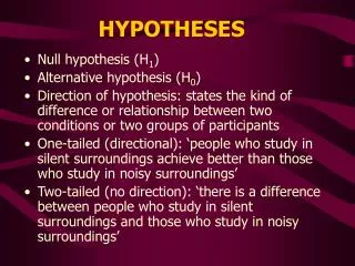
Null hypothesis testing • Difficult to evaluate specific expectations using classical null hypothesis testing: • Not always interested in null hypothesis • ‘accepting’ alternative hypothesis no answer • No direct relation • Visual inspection • Contradictory results
Null hypothesis testing • Theory • Expectations • Testing: • H0: nothing is going on vs. • H1: something is going on, but we do not know what… =catch-all hypothesis
Evaluating Informative Hypotheses • Theory • Expectations • Evaluating informative hypotheses: - Ha: theory/expectation 1 vs. - Hb: theory/expectation 2 vs. - Hc: theory/expectation 3 etc. √
Informative Hypotheses Hypothesized order constraints between statistical parameters • Order constraints: < > • Statistical parameters: means, regression coefficients, etc.
Why??? • Direct support for your expectation • Gain in power • Van de Schoot & Strohmeier, (2011), Testing informative hypotheses in SEM Increases Power. IJBD vol. 35 no. 2 180-190 7
Bayes factors for informative hypo’s • As was shown by Klugkist et al. (2005, Psych.Met.,10, 477-493), the Bayes factor (BF) of HA versus Hunc can be written as • where fi can be interpreted as a measure for model fit and ci as a measure for model complexity of Ha.
Bayes factors for informative hypo’s • Model Complexity, ci : • Can be computed before observing any data. • Determining the number of restrictions imposed on the means • The more restriction, the lower ci
Bayes factors for informative hypo’s • Model fit, fi : • After observing some data, • It quantifies the amount of agreement of the sample means with the restrictions imposed
Bayes factors for informative hypo’s • Bayesian Evaluation of Informative Hypotheses in SEM using Mplus • Van de Schoot, Hoijtink, Hallquist, & Boelen (in press). Bayesian Evaluation of inequality-constrained Hypotheses in SEM Models using Mplus. Structural Equation Modeling • Van de Schoot, Verhoeven & Hoijtink (under review). Bayesian Evaluation of Informative Hypotheses in SEM using Mplus: A Black Bear story.
Data • (1) females with a high score on negative coping strategies (n = 1429), • (2) females with a low score on negative coping strategies (n = 1532), • (3) males with a high score on negative coping strategies (n = 1545), • (4) males with a low score on negative coping strategies (n = 1072),
Model 17
Expectations • “We expected that the relation between life events on Time 1 is a stronger predictor of depression on Time 2 for girls who have a negative coping strategy than for girls with a less negative coping strategy and that the same holds for boys. Moreover, we expected that this relation is stronger for girls with a negative coping style compared to boys with a negative coping style and that the same holds for girls with a less negative coping style compared to boys with a less negative copings style.”
Expectations • Hi1 : (β1 > β2) & (β3 > β4) • Hi2 : β1 > (β2, β3) > β4)
Model 20
Bayes Factor 21
Step-by-step • we need to obtain estimates for fi and ci • Step 1. The first step is to formulate an inequality constrained hypothesis • Step 2. The second step is to compute ci. For simple order restricted hypotheses this can be done by hand.
Step-by-step • Count the number of parameters in the inequality constrained hypothesis • in our example: 4 (β1 β2 β3 β4) • Order these parameters in all possible ways: • in our example there are 4! = 4x3x2x1= 24 different ways of ordering four parameters.
Step-by-step • Count the number of possible orderings that are in line with each of the informative hypotheses: • For Hi1 (β1 > β2) & (β3 > β4) that are 6 possibilities; • For Hi2β1 > (β2, β3) > β4) that are 2 possibilities;
Step-by-step • Divide the value obtained in step 3 by the value obtained in step 2: • ci1 = 6/24 = 0.25 • ci2 = 2/24 = 0.0833 • Note that Hi2 is the most specific hypothesis and receives the smallest value for complexity.
Step-by-step • Step 3. Run the model in Mplus:
Mplus syntax DATA: FILE = data.dat; VARIABLE: NAMES ARE lif1 depr1 depr2 groups; MISSING ARE ALL (-9999); KNOWNCLASS is g(group = 1 group = 2 group = 3 group = 4); CLASSES is g(4);
Mplus syntax ANALYSIS: TYPE is mixture; ESTIMATOR = Bayes; PROCESSOR= 32;
Mplus syntax MODEL: %overall% depr2 on lif1; depr2 on depr1; lif1 with depr1; [lif1 depr1 depr2]; lif1 depr1 depr2;
Mplus syntax !save the parameter estimates for each iteration: SAVEDATA: BPARAMETERS are c:/Bayesian_results.dat;
R syntax To install MplusAutomation: R: install.packages(c("MplusAutomation")) R: library(MplusAutomation) Specify directory: R: setwd("c:/mplus_output")
R syntax Locate output file of Mplus: R: btest <- getSavedata_Bparams("output.out") Compute f1: R: testBParamCompoundConstraint (btest, "( STDYX_.G.1...DEPR2.ON.LIF_1 > STDYX_.G.2...DEPR2.ON.LIF_1) & STDYX_.G.3...DEPR2.ON.LIF_1 > TDYX_.G.4...DEPR2.ON.LIF_1)")
R syntax Compute f2: R: testBParamCompoundConstraint(btest, "( STDYX_.G.1...DEPR2.ON.LIF_1 > STDYX_.G.2...DEPR2.ON.LIF_1) & (STDYX_.G.3...DEPR2.ON.LIF_1 > STDYX_.G.4...DEPR2.ON.LIF_1) & (STDYX_.G.1...DEPR2.ON.LIF_1 > STDYX_.G.3...DEPR2.ON.LIF_1) & STDYX_.G.2...DEPR2.ON.LIF_1 > STDYX_.G.4...DEPR2.ON.LIF_1)")
Results • fi1 = .7573 • ci1= 0.25 • fi2 = .5146 • ci2 = 0.0833
Results • BF1 vsunc= .7573 / .25 = 3.03 • BF2 vsunc= .5146 / .0833 = 6.18
Results • BF1 vsunc= .7573 / .25 = 3.03 • BF2 vsunc= .5146 / .0833 = 6.18 • BF 2 vs 1 = 6.18 / 3.03 = 2.04
Conclusions • Excellent tool to include prior knowledge if available • Direct support for you expectations! • Gain in power