An Updated Associative Learning Mechanism
340 likes | 496 Views
An Updated Associative Learning Mechanism. Robert Thomson & Christian Lebiere Carnegie Mellon University. Overview. What is Associative Learning (AL) and why do we need it? History of AL implementation in ACT-R Bayesian log-likelihood transformations

An Updated Associative Learning Mechanism
E N D
Presentation Transcript
An Updated Associative Learning Mechanism Robert Thomson & Christian Lebiere Carnegie Mellon University
Overview • What is Associative Learning (AL) and why do we need it? • History of AL implementation in ACT-R • Bayesian log-likelihood transformations • From a Bayesian to Hebbian Implementation • Recent Neural Evidence: Spike Timing Dependent Plasticity • A balanced associative learning mechanism • Hebbian and anti-Hebbian associations • Interference-driven ‘decay’ • Early Results: Serial Order / Sequence Learning
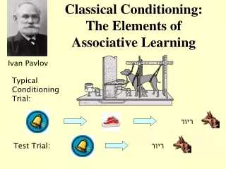
What is Associative Learning? • Associative learning is one of two major forms of learning • The other is reinforcement, although they are not necessarily distinct ‘kinds’ • It is a generalized version of classical conditioning • You mentally pair two stimuli (or a behavior and a stimulus) together • In Hebbian terms: things that fire together, wire together • ACT-R 6 currently does not have a functional associative learning mechanism implemented
Why have Associative Learning? • It instantiates many major phenomena such as: • Binding of episodic memories / context sensitivity • Anticipation of important outcomes • Non-symbolic spread of knowledge • Top-down perceptual grouping effects • Sequence Learning • Prediction Error (Rescorla-Wagner learning assumption) • It is flexible, stimulus-driven (and order-dependent) • Without associative learning it’s very hard to chain together non-symbolic information • E.g., Chunks with no overlapping slot values yet are found in similar contexts, such as learning unfamiliar sequences
History of Associative Learning in ACT-R • In ACT-R 4 (and 5), associative learning was driven by Bayesian log-odds • Association strength (sji) estimated log-likelihood of how much the presence of chunk j (the context)increases the probability that chunk iwill be retrieved
Issues with Bayesian Approach • Based on log-likelihood of recall, if two chunks (i and j) aren’t associated together, then the odds of one being recalled in the context of another is 50% • In a robust model, these chunks may have been recalled many times without being in context together • However, once these items are associated, because of the low , the odds of recalling i in the context of j ends up being much lower than if they were never associated together
Issues with Bayesian Approach Smax Sji Associative Strength 0 1 . . . -∞
ACT-R 6 Smax • Spreading Activation • Set spread (Smax) using :mas parameter • Due to log-likelihood calculation, high fan items have their sji become inhibitory • This can lead to catastrophic failure • Mature models can’t recall high-fan items due to interference Associative Strength fanji 0 Sji . . . -∞
From Bayesian to Hebbian • Really, the Bayesian approach of ACT-R 4 really isn’t that different from more neurally-inspired Hebbian learning • In both cases, stuff that fire together, wire together • When looking to update associative learning in ACT-R 6, we went to look at recent development in neural Hebbian-style learning • Recent work on spike-timing dependent plasticity inspired a re-imagination of INHIBITION in ACT-R associative learning +retrieval> ISA action light green GREEN GO retrieval DM
Traditional (Neural) Hebbian Approaches • Before getting too deep into our approach, here’s some necessary background: • Synchronous • “Neurons that fire together wire together” • Change in ∆wij is a rectangular time window • Synapse association is increased if pre- and post-synaptic neurons fire within a given temporal resolution tj j ti 1 i ∆wij 0 -∆t ∆t 0
Traditional Hebbian Approaches • Asynchronous • Change in ∆wij is a gaussian window • Very useful in sequence learning (Gerstner & van Hemmen, 1993) • Synapse association is increased if pre-synaptic spike arrives just before post-synaptic spike • Partially-causal firing tj j ti 1 ∆wij i 0 -∆t ∆t 0
Recent Neural Advances:Spike Timing Dependent Plasticity • If the pre-synaptic firing occurs just before the post-synaptic firing, we get long-term potentiation • However, if the post-synaptic firing occurs just before the pre-synaptic firing, we get long-term depression • (Anti-Hebbian Learning) • Spike-based formulation of Hebbian Learning
Neural Evidence • Post-synaptic NMDA receptors use calcium channel signal that is largest when back-prop action potential arrives shortly after the synapse was active (pre-post spiking) • Triggers LTP (similar to asynchronous Hebbian learning) • You also see the same NMDA receptors trigger LTD when the back-prop action potential arrives BEFORE the pre-synaptic synapse was active (post-pre spiking) • Seen in hippocampal CA1 neurons (Wittenberg & Wang, 2006) • This is different from GABAergic inhibitory inter-neurons, which have also been extensively studied throughout cortical regions • Which I would argues is more like partial matching / similarity
From Bayesian to Hebbian - Revisited • We’ve just reviewed some interesting evidence for timing-dependent excitation AND inhibition • Why is inhibition so important? • There needs to be a balance in activation. • It’s neurally-relevant (and necessary) • The alternatives aren’t neurally-plausible • But… we’ve waited long enough, so lets proceed to the main event:
A Balanced Associative Learning Mechanism • Instead of pre-synaptic and post-synaptic firing, we look at: • The state of the system when a retrieval request is made • The state of the system after the chunk is placed in the buffer • Hebbian learning occurs when a request is made • Anti-Hebbian learning occurs after the retrieval +retrieval> ISA action Where light color green DM GO-1 retrieval GREEN-1
Hebbian Learning Component • Initially based on a set spread (similar to :mas) divided evenly by the number of slots in the source chunk • This is subject to change as we implement into ACT-R • Ideally I’d like this to be driven by base level / pre-existing associative strength (variants of the Rescorla-Wagner learning rule and Hebbian delta rule) • Interference-driven ‘decay’ is another possibility • The sources are the contents of the buffers • One change we made was to have the sources be only the difference in context for reasons we’ll get into
Anti-Hebbian Learning Component • It’s intuitive to think that a retrieved chunk spreads activation to itself • That’s how ACT-R currently does it • However, this tends to cause the most recently-retrieved chunk to be the most likely to be retrieved again (with a similar retrieval request) • You can easily get into some pretty nasty loops where the chunk is so active you can’t retrieve any other chunk • BLI and declarative FINSTs somewhat counteract this
Anti-Hebbian Learning Component • Instead, we turned this assumption on its head! • A retrieved chunk inhibits itself, while spreading activation to associated chunks • By self-inhibiting the chunk you just retrieved, you can see how this could be applied to sequence learning • The retrieved chunks the spread activation to the next item in the sequence while inhibiting their own retrieval • This is a nice sub-symbolic / mechanistic re-construing of base-level inhibition • It also could be seen as a neural explanation for the production system matching a production then advancing to the next state
Anti-Hebbian Learning Component • The main benefit of having an inhibitory association spread is that it provides balance with the positive spread • This helps keep the strength of associations in check (i.e., from growing exponentially) for commonly retrieved chunks • Still, we haven’t spent much time saying exactly what we’re going to inhibit!
What do we Inhibit? • You could just inhibit the entire contents of the retrieved chunk • In pilot models of sequence learning, if the chunk contents weren’t very unique, then the model would tend to skip over chunks • The positive spread would be cancelled out by the negative spread • In the example to the right, assume each line is +1 or -1 spread (613) 513 - 868 6 1 3 5 1 3 RECALL 6 1 3 5 1 3 8 6 8 SA1: IN1: +3 -3 +2 -2 +1 -1 SA2: -1 +1 -1 SA3: -1 -3 +3
Context-Driven Effects • When lists have overlapping contexts (i.e., overlapping slot-values), then there are some interesting effects: • If anti-hebbian inhibition is spread to all slots, then recall tends to skip over list elements until you get a sufficiently unique context • If anti-hebbian inhibition is only spread to unique context, then there’s a smaller fan, which facilitates sequence-based recall • The amount of negative association spread is the same, the difference is just how diluted the spread is
How else could we Inhibit? • Instead, we attempted to only spread and inhibit the unique context • This sharpened the association and led to better sequence recall • As you can see, you get more distinct association in sequence learning • Essentially, you (almost) always get full inhibition of previously recalled chunk (613) 513 - 868 6 1 3 5 1 3 RECALL 6 1 3 5 1 3 8 6 8 SA1: S1: +3 +3 +2 +2 +1 +1 SA2: S2: -1 -3 +3 +1 -1 -3 SA3: S3: -1 -1 -3 -3 +3 +3
Differences from Bayesian • By moving away from log-likelihood and into a ‘pure’ hebbian learning domain, we’ve eliminated the issue of high fan items receiving negative spread • Also, this move allows us to model inhibition in a neurally-plausible manner • You can’t easily model negative likelihoods (inhibition) using a log-based notation because negative activations quickly spiral out of control • I know someone still wants to ask: why do we NEED to model inhibition?
Issues with Traditional Approaches • Traditional Hebbian learning only posited a mechanism to strengthen associations, leading modelers to deal with very high associative activations in a ‘mature’ models • You need to balance activations! • Three(ish) general balancing acts: • Squash: Fit ‘raw’ values to logistic/sigmoid type distribution • Decay: Have activations decay over time • Do Both
Squashing Association Strength • Most traditional Hebbian-style learning implementations aren’t very neurally plausible in that our brains don’t handle stronger and stronger signals as we learn • Many cell assemblies require some form of lateral inhibition to specialize • Squashing association strength, generally to a [0 to 1] or [-1 to 1] range, also isn’t very neurally plausible • Let’s look an at example:
Squashing Association Strength • It looks silly as an animation, but it’s what a lot of implementations do • Instead of squashing to a non-linear distribution, we should be trying to find a balance where associative learning is more-or-less zero sum • That’s what our mechanism attempts to do, by balancing excitatory and inhibitory associations • The goal is to specialize chunk associations by serializing/sequencing recall • Degree of association gain will be based on prior associative strength and/or base-level of involved chunks
Interference-Driven Decay • Another alternative to squashing is interference-driven ‘decay’ • ‘Decay’ based on interference due to list length • As the number of items to recall in a similar context grows, the amount of activation spread is reduced • We also have a variant based on list length and recency • Results fit an exponential decay function (on next slide) • Further work will find the balance between interference-driven and temporal-based decay • I prefer an expectancy-driven associative system where highly associated chunks won’t get a big boost • This may be modeled similar to how base-level is calculated
An Example: Serial Order Effects • Recall a list of 8 chunks of 3 elements in sequence • Assume spread of 3 • No full-chunk repetition • No within-chunk confusion ChunkAssociations ----- ------------ (8 0 6) (8 . -1.0) (0 . -1.0) (6 . -1.0) (4 . 1.0) (9 . 1.0) (1 . 1.0) (4 9 1) (4 . -1.0) (9 . -1.0) (1 . -1.0) (6 . 1.0) (7 . 1.0) (5 . 1.0) (6 7 5) (6 . -1.5) (7 . -1.5) (0 . 1.0) (5 . 2.0) (5 0 5) (0 . -1.0) (5 . -2.0) (3 . 1.0) (2 . 1.0) (4 . 1.0) (3 2 4) (2 . -1.5) (4 . -1.5)(6 . 1.0) (9 . 1.0) (3 . 1.0) (6 9 3) (6 . -3.0) (3 . 1.0) (9 . 1.0) (7 . 1.0) (3 9 7) (3 . -1.0) (9 . -1.0) (7 . -1.0)(2 . 1.0) (4 . 1.0) (6 . 1.0) (2 4 6) (2 . -1.0) (4 . -1.0) (6 . -1.0)
Serial Order: Confusion Matrix • We get serial order ‘for free’ by context-driven asynchronous spread of activation • Emergent property of model, wasn’t expected Recall Position 1 2 3 4 5 6 7 8 _ 0.865 0.025 0.015 0.015 0.005 0.020 0.030 0.025 0.000 0.780 0.030 0.050 0.045 0.025 0.035 0.035 0.025 0.005 0.710 0.045 0.050 0.070 0.050 0.045 0.025 0.055 0.010 0.645 0.045 0.065 0.085 0.070 0.015 0.040 0.080 0.030 0.585 0.065 0.090 0.095 0.025 0.045 0.080 0.090 0.045 0.540 0.070 0.105 0.020 0.040 0.045 0.090 0.120 0.045 0.545 0.095 0.020 0.055 0.050 0.055 0.085 0.135 0.075 0.525 Chunk Order
Positional Confusion • In the ACT-R 4 model of list memory, position was explicitly encoded and similarities were explicitly set between positions (set-similarities pos-3 pos-4 .7) • Interestingly, with our model of associative learning, you get some positional confusion ‘for free’ out of the asynchronous nature of the learning • You don’t get a fully-developed gaussiandropoff, but things like rehearsal and base-level decay aren’t modeled yet
Future Plans / Open Questions • How will we merge associations? • Which buffers will be sources of association and which will use associative learning? • Optimize processing costs? • Use associative learning to replicate classical-conditioning experiments • Extend to episodic-driven recall • Use association to drive analogical reasoning