EXPLICIT METHODS FOR STIFF EQUATIONS
EXPLICIT METHODS FOR STIFF EQUATIONS. C. W. Gear NEC Laboratories America (retired) Univ of Illinois at Urbana-Champaign (retired) Princeton University (part time) wgear@princeton.edu cwg@nec-labs.com Collaboration with I. G. Kevrekidis Dept of Chemical Engineering Princeton University

EXPLICIT METHODS FOR STIFF EQUATIONS
E N D
Presentation Transcript
EXPLICIT METHODS FOR STIFF EQUATIONS C. W. Gear NEC Laboratories America (retired) Univ of Illinois at Urbana-Champaign (retired) Princeton University (part time) wgear@princeton.edu cwg@nec-labs.com Collaboration with I. G. Kevrekidis Dept of Chemical Engineering Princeton University yannis@princeton.edu
Objectives of this talk • Describe some new explicit methods for stiff ODEs – they have the potential to provide large speedups for some types of problems • Discuss how they might be applied to problems in transient network analysis • Hopefully interest at least one of the audience in pursuing this further on network problems
A brief (biased) review of the early evolution of transient network analysis • Early-mid `60s: A lot of clever matrix techniques to create a system of ODEs from element specifications and Kirchoff laws • and many proposals for special methods to handle the stiff ODEs that arose • Late `60s-early `70s: Understanding that one had to use implicit methods for stiff equations and the introduction of, e.g. BDF, IRK, as general methods • Development of methods for sparse equations • Early `70s: Direct methods for Differential Algebraic Equations (DAEs) introduced to avoid the need to find the underlying ODEs • Mid `70s: View that it was better not to manipulate equations to eliminate variables since it tended to destroy sparsity, making the major task that of solving the (non-linear) equations at each time step. • Most of the computational work placed on the (non)linear equation solver
The methods to be proposed in this talk are explicit methods for ODEs. They achieve their advantage, if any, by avoiding the solution of large systems of (non-linear) equations. They do not apply (at the moment) to DAEs – and it probably will not make sense to apply them directly to DAEs because then it would be necessary to solve the non-linear equations, removing any advantage they might have.Possible difficulties: • Are the earlier methods of reduction to ODEs applicable to the current range of problems? • Do we have enough information about the behavior (e.g. time constants) of network subsections to permit use of these methods? (We will need this information) • Will other forms of computational overhead destroy any savings? If your reaction to these methods is that they will never work for these problems, I will have to respond that you are probably correct, but that we will never make progress if we don’t explore new approaches and revisit some of the approaches that were dropped in the past for reasons that may no longer be valid!
Background The methods to be described were initially developed for a type of multiscalemodeling. In that application one had a microscopic model of a system (or process) that operated over very small time scales, but one wished to look at the macroscopic behavior over long time scales and (perhaps) ignore the fine detail. Information was extracted from the detailed model and used to project forward in time (a form of extrapolation), so the method was called a projective method. It is related to some methods used for highly oscillatory problems in network analysis (see talks in this meeting), but that will not be the focus of this talk. In this talk I will focus on the favorable stability properties of these explicit methods. Some of the reports and references are available on www.neci.nj.nec.com/homepages/cwg/
Starting value Inner integration “output” points Integration processes Derivative estimate time Basic idea of projective integration We have some sort of simulation process that we call the inner integrator(explicit integration, Monte Carlo, etc.) which we run for a (short) period of time – “until the system has settled down” which can mean until unwanted stiff components have damped, or we have reached a reasonable average configuration, or … - and then we estimate the time derivatives of the variables of interest from the more recent computational results. For example, we could use the chord through the last two computed points. This estimate is used in some integration-like formula that we call the outer integrator, y
Projective Forward Euler Method - linear fit to last two points
Projective Integration We suppose we have a one-step integrator (y) that computes y(t+h) from y(t) for a the differential equation y = f(y) Starting from y0 = y(t0) we apply this k times to form y1, y2, … , yk. Now we apply it one more time and use yk and yk+1 to estimate the derivative. We then use this derivative to integrate (extrapolate) forward a distance Mh. It can be written as: yk+1+M = (M+1)yk+1 – Myk This is the Projective Forward Euler method
Projective Integration - a sequence of outer integration steps: The accuracy and stability of these methods can be studied with the usual tools. In this talk we will focus on use of extensions of these methods to get integrators that are stable in specified regions.
Stability analysis – simple case: Projective Forward Euler (PFE) Usual linear analysis: for y = ly • Assume that one step of the supplied integrator (y) (the inner integrator) has an amplification of (hl) • for Forward Euler (h) = 1+hl • for an “exact” integrator (h) = exp(hl) • Amplification of PFE from t0 to tk+1+M is • s = rk[(M+1)r – M] = rk[1 + (M+1)(r-1)] • which is rk[1 + (M+1) h] if inner is Forward Euler • Region of absolute stability: Set of r such that |s| 1. • (Note: we express stability in terms of r making independent of the form of the inner integrator - which we may not know.) • Compute stability region by finding all r such that |s| < 1 • The region of absolute stability of takes one of two forms:
M = 5 M = 7 M = 9 -plane plotk = 2, M = 5, 7, and 9 As M increases, change from one region to two. This happens when M/k ≈ 3.6 Note: = 1+h if inner integrator is Forward Euler this is usual stability plot.
If M is large: -plane [= (1+h)-plane] 1 0 Such a small stability region - what’s the point?
Consider large M: Outer Integrator step Mh: Mh - plane is one of interest for stability Asymptotically a disk of radius M(1 - 1/k) Asymptotically the stability region of the Forward Euler method -2 0 -M
For any k, and M = 0, the stability region is simply the stability region of the inner method. For fixed k, as M gets large, the stability region divides into two parts. Asymptotically in large M they are: 1. A disk around the origin of the r-plane of radius (1/M)(1/k) 2. A region that in the M(r - 1)-plane (i.e. the Mhl-plane for FE)* is the stability region of the outer integrator (the Forward Euler method in the example discussed). In other words, asymptotically we get exactly the stability we might expect for an explicit method with large step size, Mh, plus a region around the origin of the -plane. This additional region is the one we will use to damp the stiff components. * NOTE: If inner integrator is consistentthe (-1)-plane is asymptotically the same as the h-plane near the origin because (h ) = eh + O(h )2
Note that the stability region around the origin has radius (1/M)1/k • Suppose we have a problem with a gap in its spectrum - two disjoint clusters of eigenvalues: • S0 -- a disk centered at -l0 < 0 with radius l0r - the potentially stiff components • SA -- a region near the origin - the active components • If we choose h = 1/ l0 for the inner step (and use forward Euler), and if k is chosen large enough such that rk < 1/M, then the method will be stable for the cluster S0. • We can then choose an outer step commensurate with the active components in SA. • Similar results follow for higher-order methods:
First-order, explicit methods are seldom sufficiently accurate. There are several ways to get increased accuracy: (i) use the inner integrator a further q times after yk and project forward using a q-th order polynomial extrapolation through yk, yk+1, … , yk+q (ii) use information from several past groups of inner steps in a multistep-like integrator (iii) use implicit methods (but in an explicit manner – will not be discussed further today)
Approximately 1/M Stability Region of 4th order R-K method Radius about (q!/Mq)1/k A 4-th order method: Stability region: k=4, q=4, M=10
What good is a couple of Stability Regions? • Typical problem has lots of eigenvalues that could be: • Spread in an unknown fashion in the negative half plane • In moderately well known clusters – each due to the time constant(s) of a particular subsystem but there could be many such clusters • Have negative real parts but with significant imaginary parts • How do we handle these situations with this simple method?
Telescoping Projective Methods (handling multiple clusters of eigenvalues) We have created an “outer integrator” over a step size of h(k+q+M) using an inner integrator over step size h. Why not use recursion? (really iteration) Let the inner integrator be 0 First level outer integrator is 1e.g., for Projective Euler 1 = 0k((M+1) 0 - M) Projective integrator based on i is i+1 i+1 = ik((M+1) i - M) for PFE (if k and M are fixed) It uses step size h(k+q+M)i+1 - growing exponentially, or, more generally, hi+1 = (ki + qi + Mi)hi
One outer integrator step - 1 Projective Forward Euler Method - linear fit to last two points
y0 y3+M y6+2M y9+3M 2 Two-level Projection method (k = 2 at both levels)
Let us consider the stability of Telescopic methods. No need to use same method at each level, or same k and M at each level, but to illustrate concepts we will start by considering the use of (projective) forward Euler at all levels. In practice, we will use first-order methods at all levels except for the outermost level since at the inner levels the step size/method is determined by stability only. At the outer level the step size/method must be chosen for accuracy.
Telescoping Projective Methods: What is stability? Consider Projective Forward Euler. Let amplification of level i integrator be i We have i+1 = ik[(M + 1)i - M] Stability region is set of that remain in unit disk (or, remain bounded) in iteration k[(M + 1) - M] This stability region will contain the stability region of the method with any finite number of iterations.
10 iterations of PFE with k=2, M=3. Outer stepsize is 60,466,176h0 As # iterations boundary becomes fractal Note that M is small so that [0,1] (or [-1,0]) is inside the stability region In this case, the stability boundary touches the real axis 10 times. Use of a slightly smaller M would place [-,1) in the interior of the stability region.
We can show that for any M there is a k0 such that for all k k0 the stability region includes the negative axis from 0 to 1 in the r-plane in the case of the Forward Euler method. In some ways, these are like high-stage number Runge Kutta Methods which have been used to extend the region of stability. (The previous slide’s 10-level projective integrator is a 59049-stage RK method!) A more interesting application may be to problems with multiple clusters of eigenvalues as shown on the next slide:
… by choosing an inner step size of 1/l0 and then using an effective step size at the outer levels of projective integration of 1/li for the i-th level we can choose values for ki (the number of steps at the (i -1)-st level before projecting at the i-th level to achieve stability over these disks. The step size at the i-th level is defined as hi = hi-1(ki-1 + Mi-1+ 1) A particular case with h = 1, 11, and 121 is shown in the next slide:
A two-level PFE2-9 method 3 stability regions determined by the 3 stepsizes: Inner 1st level 2nd level These regions are due to k (2) and cannot be placed where needed.
In effect, each successive stepsize damps eigenvalues of the order of the inverse of that stepsize. Thus, if we know where the “stiff” eigenvalues are, we can select a sequence of stepsizes to damp them. In a sense, this method is a little like using a Chebshev type iteration to remove eigencomponents in decreasing order of size, except that it is spread out over many steps. (If the problem is highly non-linear in a way that cause the eigendirections to change rapidly, more iterations (that is, inner steps) are needed, and the method becomes less efficient.
NOTE • A telescopic method is NOT the same as using a collection of different step sizes. The telescopic method can be designed so that the number of steps at any given level before a projective step is determined solely by the ratio of the step sizes at the two adjacent levels, independent of the number of levels of telescoping. • If, on the other hand, just a collection of step sizes are used, more smaller steps are needed as the size of the largest step increases.
What about complex eigenvalues?Use some sort of two-stage method (RK-like) which will have (h) = 0 when h has complex conjugate values (if used as the inner integrator) or () = 0 when has complex conjugate values for intermediate stage integrators..For example, This has which has roots at and are complex for r = > 1/4. (Second order if r = 1/2.)
Similar technique can be used for intermediate level projective step. Alternatively (and more simply) one can use k+2 inner steps and then do a projective step using the last three points in: yk+2+M =rM2yk+2+(M-2rM2)yk+1 -(M-1-rM2)yk to achieve a stability polynomial of the form = k[1 + M(-1) + rM2 (-1)2] This places stability regions around the complex conjugate eigenpair given on the last slide. With this technique we can place regions of stability around any desired sets of locations in the complex plain, as shown in the next slide.
Stability plot of 4-level projective method in the = 1+h0 plane. The sizes of steps at each level are h0, 4h0, 20h0, 80h0, and 880h0. The outermost is Projective Forward Euler (k=1, M=9), so the right-most region - a dot in the figure at (0,1) is near the stability region for the forward Euler with step size 880h0. The first and third levels used the method on the last slide with r=0.3 and r=0.35 respectively (with k=1, M=3) to place stability regions around 0.440.25i, and 0.9760.015i respectively. The second level was PFE with k=1, M=3 placing a region near 0.95. Larger values of k would make the regions (except for the rightmost) larger.
Concluding remarks • if eigenvalue locations are known (or can be estimated on the fly), and • if we can reduce the system to ODE’s these methods may be able to save significant time because no large systems have to be solved. Because method is explicit, “subcycling” (also known as multirate methods – different time steps for different components) is easier to apply. If certain eigenvalue groups are isolated in subparts of the network, it may be possible to restrict the use of the stepsizes designed to damp those eigenvalues just to those subnetworks.