Download
1 / 31
320 likes | 439 Views
Lecture 8: Risk Modelling Insurance Company Asset-Liability. What we will learn in this lecture. We will build a simplified model of the insurance company’s portfolio of assets and liabilities We will look at how this model is an extension of the classical mean-variance model

E N D
What we will learn in this lecture • We will build a simplified model of the insurance company’s portfolio of assets and liabilities • We will look at how this model is an extension of the classical mean-variance model • We will look at how the optimal portfolio is dependant upon the leverage • We will generate a locus of frontiers for various leverage levels
A Recap of the Mean-Variance Model • We can describe the stochastic behaviour of a portfolio in terms of the stochastic behaviour of the assets it contains • Assets are purchased in the initial period and sold or valued for an unknown price in the future • The value of assets purchased is equal to our initial wealth (ie no short sales or leverage) • Some combinations of assets are superior to others leading to the concept of efficient portfolios and frontiers
The Idea of a Stochastic Asset • The stochastic asset can be viewed as a box in which you put a fixed amount of money into and take a variable or stochastic amount of money out Asset Held For Period of Time Fixed Amount Invested Variable Amount Taken Out
The Idea of Leverage • Leverage can be viewed as a box in which you take an initial amount of money out and at a later date must return a fixed amount. Leverage Held for a Fixed Period Fixed Amount Taken Out Fixed Amount Paid Back Time
The Idea of a Stochastic Liability • The stochastic liability can be viewed as a box in which you take a fixed amount of money out and at a future period put a variable money Liability held for a fixed time Fixed amount taken out Variable amount paid back Time
Liabilities Are A Form Of Leverage • Like leverage, liabilities provide an initial income stream which can be invested in assets • So if you have £100 in wealth and sell £100 of liabilities you will have £200 to invest • However the amount you will have to pay back in the future on the £100 of liabilities is variable
A Diagram Of Leverage Through Stochastic Liabilities Liability Held For Fixed Time Fixed Capital From Liabilities Sold Variable Payment Made On Liabilities Investment Through Wealth Assets Held For Fixed Time Variable Remaining Wealth Fixed Capital Invested From Wealth and Liabilities Sold Variable Value of Asset Time
In Equation Form • Total value of asset purchased in an initial time period equals the sum of wealth invested plus value of liabilities sold: A0 = L0 + W0 where A0 is the value of assets, L0 is liabilities and W0 is wealth all at initial time 0 • Likewise the future value of assets is split between liabilities and wealth: A1 - L1 = W1 Or A1 = L1 + W1 A1 is the value of assets, L1 is liabilities and W1 is wealth all at initial time 1 • Therefore changes can in wealth can be expressed: (W1 – W0) = (A1 – A0)- (L1 – L0)
The Kahane Model • The Kahane Model is adapts the Mean Variance framework to the describe the statistical properties of an insurance companies portfolio of assets and liabilities • The key observation of the Kahane Model is that insurance business written is essentially a stochastic liability with which the insurance company levers its asset portfolio
Stochastic Insurance Liabilities • Insurance liability contracts are identical to generic stochastic liabilities • The initial payment received from the liability is the premium • The obligatory claim made to the liability is the claim • We will build our model assuming zero costs and reinsurance, but latter relax this assumption • Therefore the initial payment towards the stochastic liability is gross premiums and the obligatory outflow payment is gross claims
Insurance Liability Contract Diagram • Insurance liability contracts provide an initial payment to the insurance company of Gross Premiums • The Insurance Company is obliged to pay a future payment equal to Gross Claims Insurance Liability Contract Gross Claims Gross Premiums Time
The Equations of The Kahane Model • The level of assets invested by the insurance company at time 0 is equal to shareholder funds plus premiums from insurance contracts: SAi0 = Si0 + SPi0 where Ai0 is ith assets, S0 is shareholder funds and Pi0 is the premium on the ith insurance business all at time 0 • This can be rewritten as proportions of shareholder funds: 1 = S(Ai0/S)– S(Pi0/S) • We will express these as weights 1 = SWAi0 – SWPi0 Where WAi0 is the proportion of shareholder funds invested in the asset ith at time WPi0 is the proportion of shareholder funds to premiums from the ith insurance line
The Equations of The Kahane Model Continued • Taking the system of equations forward to period 1 S1 = SAi1 – SCi1 Where S1 is shareholder funds in period 1, Ai1 is the value of the ith asset in period 1 and Ci1 is the value of the ith asset in period 1 • Where Ai1 = Ai0.eri Ci1 = Pi0.Vi where ri is the return on the ith asset and Vi is the gross claims ratio on the ith insurance line • S1 – S0 = S(Ai1 – Ai0)+ S(Pi0 - Ci) • S1 – S0 = SAi0.(eri– 1)+ SPi0.(1 - Vi) • (S1 – S0 ) / S0 = S (Ai0/S0).(eri– 1)+ S (Pi0/S0). (1 - Vi) • RS = S WAi0.RAi + S WPi0.RLi (KEY EQUATION!) where RAi is the return on the ith asset, RLi is the return on the ith insurance liabilities defined as 1 - Gross Claims Ratio and RS is the return on shareholder funds all across the defined period
Insurance Liability Profit = Premium – Claim Profit = Premium * (1 – Gross Claim Ratio) Return = (1 – Gross Claim Ratio) Insurance Premium Insurance Claim Insurance Contract Time
The 1 Asset 1 Liability case • For an insurance company with 1 asset and 1 liability RS = WA10.RA1 + WP10.RC1 • The expected return on shareholder funds: E(RS) = E(WA10. RA1+ WP10.RL1) E(RS) = WA10.E(RA1) + WP10.E(RL1) • The variance of return on shareholder funds: Var(RS) = E(WA10. RA1+ WP10.RL1) Var(RS) = WA102.Var(RA1) + WP102. Var(RL1) + 2. WA10. WP10 .Cov(RA1, RL1) • Where WA – WL = 1.0 and WA > 0 WL > 0
Generalized Matrix Form For Weight Matrix W = W is the weight vector WAi is the weight invested in the ith asset as a proportion of shareholder funds WLi is the weight invested in the ith liability as a proportion of shareholder funds
Generalized Form For the Expected Return Matrix R = R is the expected return vector E[RAi] is the expected return on the ith asset E[RLi] is the expected return on the ith liability, as defined by 1 – Gross Claims Ratio
Generalised Matrix Form for the Covariance Matrix C = Var(RAi) is the variance of return on the ith asset Var(RLi) is the variance of return on the ith liability Cov(RAi,, RAj) is the covariance of return between the ith and jth asset Cov(RLi,, RLj) is the covariance of return between the ith and jth liability Cov(RAi,, RLj) is the covariance of return between the ith asset and jth liability
The Optimisation • Min WT.C.W subject to WT.R = Target Return WiA>= 0 for all i WiL >= 0 for all i SWiA – SWiL = 1 • Problem: leverage is unconstrained, no limit on the level of insurance contract liabilities we use to lever our portfolio
The Leverage Constraint • Regulation constrains the maximum level of insurance liabilities sold and compared to the insurance companies base capital. • We will express this relationship as: S Pi <= a.S where Pi is the gross premium sold of the ith insurance liability contract, S is the level of shareholder capital and a is leverage constraint imposed by regulation • This can be re-express as: S (Pi/S) <= a • WPi <= a
The Complete Kahane Optimisation Problem • Min WT.C.W subject to WT.R = Target Return WiA>= 0 for all i WiL >= 0 for all i SWiA – SWiL = 1 SWiL <= a • Notice how the level of leverage must also be chosen
The Kahane Efficient Frontier • The Kahane model provides the insight that an insurance company’s efficient portfolio is not just dependant upon an optimal set of portfolio weights • It is also dependant upon on the selection an optimal level of leverage. • In optimal low variance portfolios will have a low leverage, high return optimal portfolios will have a high leverage. • For each level of leverage there is a unique efficient frontier, however some levels of leverage provide a more efficient way of achieving a desired return
Multiple Frontiers for Different Leverage Levels Crossover from one frontier to the next Increasing Leverage Expected Return Increasing Maximum Return with leverage Increasing Minimum Variance with leverage Portfolio Standard Deviation
Insurance Asset Liability Frontier As An Envelope of Sub-Frontiers • The efficient frontier for the insurance company’s asset-liability portfolio is the envelope of the various sub-frontiers for various leverage levels • The Envelope frontier is calculated by taking the minimum risk for a given level of return across all the frontiers • We are taking the optimal frontier at that return level.
Envelope Frontier Envelope Frontier made up from sections of the sub-frontiers Increasing Leverage Expected Return Sub-frontiers for different leverages Portfolio Standard Deviation
Extensions to the Model • The first assumption that needs extending is the way in which we calculate the return on insurance claims liabilities • In reality the insurance company has reinsurance costs and broker costs • We can capture this by changing the way we measure the return on liabilities
A More Realistic Stochastic Claims Liability Variable Amount of Claims Paid Net of Reinsurance Fixed Amount Given to the Insurance Company Fixed Amount Gross Premiums Sold Fixed Amount of Broker fees and Reinsurance Costs Paid out • We estimate the returns on this more complicated system by using net premiums written minus broker cost to net claims incurred (an adjusted net claims ratio) • RLi = 1 –NCi where RLi is the adjusted return on the ith insurance liability and NCi is the adjust net claims ratio on the ith line of business
Dealing With Claims Liabilities Runoff Patterns • So far we have modelled insurance claims liabilities as a system providing a fixed income of capital at an initial time and requiring a stochastic payment of capital at some future point • In reality it requires a stochastic stream of future payments related to the runoff pattern • One way of dealing with this complex problem it to take the time weighted average of the future cash flows and assume a single payment is required at this point
Diagram of Time Weighted Average of Cash Flow Real Runoff Pattern Across Time Time Simplified, Single Time Weight Average Payment
Using the Kahane Model To Calculate VaR on Shareholder funds • Since the Kahane model allow us to ultimately calculate the expected return and variance of shareholder funds it can be used to calculate the VaR on shareholder funds • However it would be necessary to adjust expected returns on insurance liabilities into their continuously compounded form so they could be scaled across time.