Download

1 / 23
240 likes | 380 Views
ARCH and GARCH Vaibhav Gupta MIB, Doc, DSE, DU. REFS RISK AND VOLATILITY: ECONOMETRIC MODELS AND FINANCIAL PRACTICE Nobel Lecture, December 8, 2003 Robert F. Engle III. Introduction. Advantage of knowing about risks: You can change your behaviour to avoid it.

E N D
REFS RISK AND VOLATILITY: ECONOMETRIC MODELS AND FINANCIAL PRACTICE Nobel Lecture, December 8, 2003 Robert F. Engle III
Introduction • Advantage of knowing about risks: You can change your behaviour to avoid it. • To avoid all risks would be impossible: no flying, no driving, no walking, eating, drinking, no to sunshine. To some who are obsessed with a early morning bath, NO BATH as well. • There are some risks we choose to take because the benefits exceed the costs. • Optimal behaviour takes risks that are worthwhile. • This is central paradigm to finance. • Thus we optimize our behaviour, in particular our portfolio, to maximize rewards and minimize risks.
Simple Concept of Risk can mean a lot of nobel citations • Markowitz (1952) and Tobin (1958) associated risk with the variance in the value of a portfolio: From the avoidance of risk they derived optimizing portfolio and banking behaviour. (Nobel Prize 1981) • Sharpe (1964) developed the implications when all investors follow the same objectives with the same information. This theory is called the Capital Asset Pricing Model or CAPM, CAPM, and shows that there is a natural relation between expected returns and variance. (Nobel Prize 1990)
Black and Scholes (1972) and Merton (1973) developed a model to evaluate the pricing of options. (1997 Nobel Prize)
Typically the square root of the variance, called the volatility, was reported. They immediately recognized that the volatilities were changing over time. • A simple approach, sometimes called historical volatility, was and widely used. (sample standard deviations over a short period) • What is the right period: • Too long: Not relevant for today • Too short: Very noisy • Furthermore, it is volatility over a future period that should be considered as risk, forecast also needed in the measure of today. • Theory of dynamic volatility is needed: ARCH
Until the early 80s econometrics had focused almost solely on modelling the means of series, i.e. their actual values. Recently however we have focused increasingly on the importance of volatility, its determinates and its effects on mean values. • A key distinction is between the conditional and unconditional variance. • the unconditional variance is just the standard measure of the variance • var(x) =E(x -E(x))2
the conditional variance is the measure of our uncertainty about a variable given a model and an information set. cond var(x) =E(x-E(x| ))2 Conditional variance this is the true measure of uncertainty variance mean
Stylised Facts of asset returns i) Thick tails, they tend to be leptokurtic ii)Volatility clustering, Mandelbrot, ‘large changes tend to be followed by large changes of either sign’ iii)Leverage Effects, refers to the tendency for changes in stock prices to be negatively correlated with changes in volatility. iv)Non-trading period effects. when a market is closed information seems to accumulate at a different rate to when it is open. eg stock price volatility on Monday is not three times the volatility on Tuesday. v) Forcastable events, volatility is high at regular times such as news announcements or other expected events, or even at certain times of day, eg less volatile in the early afternoon.
vi) Co-movements in volatility. There is considerable evidence that volatility is positively correlated across assets in a market and even across markets
Engle(1982) ARCH Model Auto-Regressive Conditional Heteroscedasticity an AR(q) model for squared innovations.
note as we are dealing with a variance even though the errors may be serially uncorrelated they are not independent, there will be volatility clustering and fat tails. if the standardised residuals are normal then the fourth moment for an ARCH(1) is
Volatility • Volatility – conditional variance of the process • Don’t observe this quantity directly (only one observation at each time point) • Common features • Serially uncorrelated but a depended process • Stationary • Clusters of low and high volatility • Tends to evolve over time with jumps being rare • Asymmetric as a function of market increases or market decreases
The basic models • Consider a process r(t) where Conditional mean evolves as an ARMA process How does the conditional variance evolve?
Modeling the volatility • Evolution of the conditional variance follows to basic sets of models • The evolution is set by a fixed equation (ARCH, GARCH,…) • The evolution is driven by a stochastic equation (stochastic volatility models). • Notation: • a(t)=shock or mean-corrected return; • is the positive square root of the volatility
ARCH model • We have the general format as before • The equation defining the evolution of the volatility (conditional variance) is an AR(m) process. Why would this model yield “volatility clustering”?
Basic properties ARCH(1) Unconditional mean is 0.
Basic properties, ARCH(1) Unconditional variance What constraint does this put on 1?
Basic properties of ARCH • 01<1 • Higher order moments lead to additional constraints on the parameters • Finite positive (always the case) fourth moments requires 0 12<1/3 • Moment conditions get more difficult as the order increases – see general framework of equation 3.6 • Note – in general the kurtosis for a(t) is greater than 3 even if the ARCH model is built from normal random variates. • Thus the tails are heavier and you expect more “outliers” than “normal”.
ARCH Estimation, Model Fitting and Forecasting • MLE for normal and t-dist ’s is given on pages 88 and 89. • The full likelihood is very difficult and thus the conditional likelihood is most generally used. • The conditional likelihood ignores the component of the likelihood that involves unobserved values (in other words, obs 1 through m) • MLE for joint estimation of parameters and degree of the t-distribution is given. • Model selection • Fit ARMA model to mean structure • Review PACF to identify order of ARCH • Check the standardized residuals – should be WN • Forecasting – identical to AR forecasting but we forecast volatility first and then forecast the process.
GARCH model • Generalize the ARCH model by including an MA component in the model for the volatility or the conditional variance. Proceed as before – using all you learned from ARMA models.