Download
1 / 125
1.25k likes | 1.41k Views
NRAO June 27-30, 2004. SARA 2004 CONFERENCE. Plasma Bubble Detection & Analysis at 20 MHz. Professor John C. Mannone Professor Wanda Diaz Central Piedmont Community College University of Puerto Rico Duke-Cogema-Stone & Webster Department of Physics

E N D
NRAO June 27-30, 2004 SARA 2004 CONFERENCE
Plasma Bubble Detection & Analysis at 20 MHz Professor John C. Mannone Professor Wanda Diaz Central Piedmont Community College University of Puerto Rico Duke-Cogema-Stone & Webster Department of Physics Charlotte, NC San Juan, Puerto Rico
Spectral Analysis Techniques Developed SARA Conference July 2003 Solar Physics with 20 MHz Antennas Focus on Solar Flares Understanding Solar Radio Propagation Encounters Frequency Analysis Computer Simulation Website Creation Sept 2003 NASA/Radio Jove Bulletin Article October 2003 ORION Lecture October 2003 Solar-Ionosphere Connection Simultaneous Comparative Solar Burst Analysis Development of Radio Scintillation Experiments SARA Conference June 2004 Plasma Bubble Detection & Analysis
"DETECTION AND ANALYSIS OF PLASMA BUBBLES AT 20 MHz RADIO FREQUENCY" ABSTRACT Charge deficient holes in the F-region, called plasma bubbles, are typically detected above the equatorial zone. Some of the traditional techniques of detection involve sensitive receivers called riometers tuned to 30 MHz to record time variations or rocket-borne Langmuir probes measure the fluctuation of electron number density.In this work, the electron number density variations are recorded indirectly. Astrophysical radio waves are modulated by these variations as they travel through the ionosphere. Spectral analysis of decametric radio signals acquired with 20 MHz antennas will provide similar information about the ionosphere. The behavior of the radio noise floor will show if radio light is scintillated. This technique is applied to data from Puerto Rico. Though just north of the magnetic equatorial zone,power spectra disclose radio twinkling by the sudden post-sunset onset of plasma bubbles just before local midnight.
Irregularities and Radio Scintillation Optical Twinkle- Variation refractive index caused by fluctuations in mass density in the turbulent atmosphere (troposphere) Radio Twinkle- caused by random fluctuations in electron number density in the ionosphere Important in Navigation Communication Pulsar Research
Science & Industry Radio Scintillation Detection 30 MHz Riometer- very sensitive low noise receiver and 4-element Yagi arrays Radar Backscatter Satellite Transmission- FLEETSAT (254 MHz), GPS Satellites (~1.2 - 1.6 MHz) Rockets Instrumented with Langmuir Probes- ne fluctuations Global UV Imager maps ionospheric ions fluctuations (volume emission rate in the far UV at 135.6 nm, due to the radiative recombination of the F-layer predominant ion O+, is proportional to ne2)
Our Methodology on Radio Scintillation Detection The extent of amplitude modulation of 20 MHz galactic radio background noise by the medium in its path(not necessarily restricted to the ionosphere) is determined and compared with known characteristics. The signal is too noisy to see the scintillations directly with the simple inexpensive receiver and phased array dipoles used; however, spectral analysis reveals the behavior of the noise floor. In concert with additional information, such as the time and location of the disturbance, geomagnetic activity, space weather, etc., the spectral analysis is a good tool that will help determine or corroborate the state of the ionosphere. The Ionosphere is a Plasma
Radio Emission Mechanisms Continuous Thermal (Coulomb Scattering) Non-thermal (Synchrotron Radiation) Discrete Atom Transitions (High Rydberg States) Hyperfine Transition ( 21 cm spin-flip) Molecular Transitions (methanol lines; water masers)
Adapted from Fig. 6.2 Atmospheric Window and Sky Brightness (NRAO library) p = -0.65 Radio Spectra of Various Sources 20 Frequency, MHz
Anatomy of the Ionosphere Layout, Composition, Formation Dynamics of Fields and Sources (g, E, B, v, P, m, n, j) Connectivity/Nonlinear Dynamics Boundary Flows/Shocks Space Weather/Terrestrial Weather (El Nina South Atlantic Oscillation, Hurricanes) Diurnal, Seasonal, Solar Cycle Effects
Exosphere (space weather) 40,000 miles / 64,400km (contains Plasmasphere & Magnetosphere) Mesosphere 50 miles / 80km Thermosphere 400 miles /640km (Ionosphere straddle these two spheres) Stratosphere ~30 miles / 50km Troposphere (neutral atmosphere/weather) 5 miles / 8.1km at poles 10 miles / 16.1km at equator
Solar Wind Deforms Earths Dipolar Magnetic Field A constant stream of particles flowing 106 mph from the Sun’s corona extends beyond Pluto’s orbit.
(106 cm3 = 1 m3 ) Note: green line is for Martian ionosphere Chapman profile 120 km, max ne = 5x104cm-3 Ionospheric Plasma Formed from complex collision dynamics and photo-ionization of air molecules involving cosmic rays and UV light.
Transparency of Earth’s Atmosphere O2 and N2 absorb all l < 290 nmH2O and CO2 block 10m to 1 cm Universe, 5th ed. Kaufmann and Friedman
Electron Plasma Frequency- Radio Wave Passage Or the Langmuir Frequency of Plasma Oscillation wpe = (4pe2n0/me)1/2 ~15 MHz on the day side of the earth near sunspot maximum and ~10 MHz on the night side near sunspot minimum Layer opaque to all lower frequencies
Significant Ionospheric Scintillation of Radio Waves Caused by Plasma Instabilities Polar/Auroral Zone Particle Precipitation Equatorial Zone Plasma Plumes and Bubbles Mid Latitudes Storm Enhanced Density (SED) from high latitudes Sudden Storm Enhancement (SSE) from low latitudes
Plasma Plumes and Bubbles Equatorial ionosphere illustration Coupled Ionosphere-thermosphere forecast model Linked to theoretical growth-rate model (left) Linked to non-linear plasma bubble evolution (right)
Rayleigh-Taylor Instability & E x B Drift
Improved version over Radio Jove RJ1.1 receiver, the RF-2001A is used here (also designed by RF Associates, Dick Flagg) Local oscillator generates a waveform at frequency around 20.1 MHz. The range of frequencies to tune at 19.950-20.250. The JFET transistor amplify incoming signals by a factor of 10. The receiver input circuitry is designed for a 50 Ohm antenna. The double dipole antenna ( Radio JOVE) is 10 feet above the ground, aligned east-west, in-phase so the beam is directly overhead. The maximum gain for a horizontal dipole is 7.3 dBi. Beam width is 115 degrees. The VSWR is below 1.5:1 Receiver noise figure < 5dB ( 620K). At the operating frequency of 20.1 MHz the galactic background temperature on the order of 50,000 degrees (this is consistent with the plasma temperature vs. ne chart).
Can Equatorial Plasma Bubbles be Detected? Phenomena normally in the equatorial zone +/- 20 degrees from the magnetic equator Most southern participating site is Puerto Rico with Geographic latitude 18.3N, but Geomagnetic latitude 28.2 N Data was collected hourly for a period before sunset to after sunrise (6 AM to 6 PM Atlantic Standard Time). Arbitrarily, the antenna signal was sampled for the first 10 minutes of each hour. The sampling rate was 1 Hz. Though the bubbles only survive around 30 minutes, the antenna is seeing numerous irregularities. (Future experiments will acquire more data over a shorter time interval and at a higher sampling rate).
Greatly exaggerated for clarity Plasma irregularity Radio wave path Simple trigonometry => sin(q-b)/sin(p-q) = R/(R + z) z 3 dB • is angle between the vertical and the half power antenna beam width • b is the maximum latitude displacement • To see an irregularity at height z (typically 600 km) • R is the radius of Earth: 6378 km q Antenna site Latitude of zenith point R b
Questionably in the Zone: need 8 degrees (28-8 = 20), may only have 3 degrees latitude E-W phased dipole array with a 60 degree full beam width and disturbance at 600 or 1100 km, allows no more than 2.8 or 4.8 degrees latitude difference, respectively. (E-W anti-phase arrangement is preferred allowing 13-19.5 degree reprieve) This configuration falls short. However, a free dipole array was assumed. With the antenna 10 ft (3 m) above the ground (1/5-wavelength), the antenna pattern may become distorted. Though less sensitive, it may now see into the equatorial zone similarly to the anti-phase capability. Dipole pattern free space vs. close to the ground
Preliminary Data Reduction Sequence • Radio Skypipe Pro software SPD files converted to TXT files • -Save data in Word document which automatically delimits the data into 3 columns: date, time, signal strength • -Correct logging errors • (37:.94 must be changed to 37:0.94; • often jumps at the minute intervals; other errors in format or placement) • -Copy data into Excel and format illegible data Data Collection &Preparation
-Note that Excel truncates the Hour in Column B. Therefore, label column as time, min:sec after the hour (e.g., after 22Z). However, computations in Excel will treat this a fractional day. -Compute sampling interval time (in seconds) in cell D4 type (=(B4-B3)*24*3600) -Plot Signal Strength vs. Time to reproduce the time series. -Compute sampling statistics -Load FFT capability in Excel by executing the submenu path Tools/Add-Ins/check Analysis Toolpak/OK -Excel algorithms require exactly 2N data points for FFT, Use 512. 1024, etc not to exceed 4096.. Truncate or pad as necessary. Sampling Statistics
-Perform FFT (Tools/Data Analysis/Fourier Analysis/OK): Input the range of data for the signal strength matching 2N points; e.g., C4:C515; direct output, e.g., F4:F515 -Decimate the frequency according to N. That is, step-wise increase the frequency (sampling frequency/N). -Calculate spectral power: square the magnitude of the complex number returned by the FFT (=IMABS(F4)2); propagate to N/2 -1 points to avoid reflection of results. -Plot Power Spectrum: Power vs. Frequency. -Scale the plot down by a factor of around 104 to105 to see the spectral components above the noise. -Plot Log Power vs. Log Frequency with close attention to the 100 to 1000 millihertz range for behavior of the noise floor. Spectral Analysis
Left Portion of Excel Spreadsheet Analysis Spreadsheet Calculations
The frequency is stepped in about 2 mHz increments (step = sampling frequency/N = 990 mHz/512 samples) Right Portion of Excel Spreadsheet Analysis Spreadsheet Calculations
20 MHz Radio Background Noise University of Puerto Rico, June 6, 2004 11 PM local time Apparently uneventful radio noise, just a dc off-set Signal Strength vs. Time Graph Reconstruction in Excel 10 minute time series sampled at 1 Hz (990 +/- 7 mHz)
Typical Power Spectral Density (Power vs. Frequency) not very revealing except for ringing
Diffraction and Scattering Models p1 Scintillation caused by change in refractive index, n, caused by diffraction on irregularities related to electron number density fluctuations or atmospheric turbulence. (Appleton-Hartree equation) Irregularity size >> wavelength, wave front is disturbed, get random phase modulation; further modulation occurs before it reaches the antenna => complicated diffraction pattern. Temporal variation if source is moving relative to the receiver.
Diffraction and Scattering Models p2 Phase screen, simplest model: irregular layer replace by equivalent thin screen a distance z to the antenna (multiple screen are necessary for extended medium and an inhomogeneous background). Fresnel Diffraction leads to power law frequency dependence f-pwhere p is the spectral index. Various types of scintillation lead to different spectral indices: the quiet sky 0.65, typical ionospheric scintillation 8/3 (2.5), plasma bubbles range 2-8 with average 4, tropospheric scintillation 11/3, interstellar scintillation like ionospheric without the seasonal or geographic restrictions.
Spectral Analysis Fresnel Zone Speed of rising plasma bubble is estimated from the corner frequency fc: (V = (lz)1/2 fc) Spectral Index, p obtained from log Power vs. log frequency plot after the roll-off (around 50 millihertz) to about 1 Hz or perhaps 2 or 3 for very strong scintillation (cut-off frequency for Fresnel filtering). Therefore, spectral behavior is examined from about 100-1000 millihertz. S4, Scintillation Index (normalized time averaged signal strength) (not a good index for our experiment since our receiver is not sensitive like a riometer).
Spectral index p = 4 for plasma bubbles over Varanasi, India Ionospheric Plasma by VHF Waves, R.P. Patel, et al Pramana Journal of Physics, India Academy of Sciences, Vol 55, No. 5 & 6, Nov/Dec 2000, pp. 699-705
Spectral index p = 5 for plasma bubbles over San Juan, Puerto Rico
Before and After the Irregularity log power vs. log frequency
Time Variation of Spectral Index June 6, 2004 6 PM June 7, 2004 8 PM 9 PM 11 PM 6 AM June 6, 2004 sunset 6:57 PM 23Z = -01Z 6/7/04 June 7, 2004 sunrise 5:48 AM = +10Z 6/7/04
Significant change in slope suggests multiple phenomena 50 100 1000 mHz Corner frequency 316 mHz relates to the first Fresnel zone Size and speed of irregularity can be estimated from this
A major change is indicated in the condition of the ionized layer during the measurement interval. Each linear segment is analyzed between 100 and 1000 mHz, the correct range for scintillation observations (the “trend line” feature in Excel is used to obtain an unbiased linear regression)
Diurnal Variation of Plasma Bubble Growth Radio sky background spectral index -0.65 Post-sunset (-01Z) and Pre-midnight (+04Z) Growth of Suspected Plasma Bubble
View of Eastern Sky/Milky Way from Puerto Rico June 6, 2004 11 PM
Geomagnetic Activity May Enhance the Occurrence of Irregularities in the Mid-latitude Region
Geomagnetic coordinate treated in this page is "geomagnetic dipole coordinate" referring to the geocentric dipole field approximating the geomagnetic field based on International Geomagnetic Reference Field (IGRF). The poles are the intersections of the dipole axis with the Earth's surface at (79.5N, 71.6W) and (79.5S, 108.4E)(IGRF 2000), and move slowly according to "secular variation of the geomagnetic field". Geomagnetic latitude and longitude are defined as shown in the illustration.