
Evaluating Predictive Models
E N D
Presentation Transcript
Evaluating Predictive Models Niels Peek Department of Medical Informatics Academic Medical Center University of Amsterdam
Outline • Model evaluation basics • Performance measures • Evaluation tasks • Model selection • Performance assessment • Model comparison • Summary
Basic evaluation procedure • Choose performance measure • Choose evaluation design • Build model • Estimate performance • Quantify uncertainty
Basic evaluation procedure • Choose performance measure (e.g. error rate) • Choose evaluation design (e.g. split sample) • Build model(e.g. decision tree) • Estimate performance(e.g. compute test sample error rate) • Quantify uncertainty(e.g. estimate confidence interval)
Probability that a given x is misclassified by h Error rate The error rate (misclassification rate, inaccuracy) of a given classifier h is the probability that h will misclassify an arbitrary instance x :
Expectation over instances x randomly drawn from Rm Error rate The error rate (misclassification rate, inaccuracy) of a given classifier h is the probability that h will misclassify an arbitrary instance x :
Sample error rate Let S = {(xi , yi) | i =1,...,n } be a sample of independent and identically distributed (i.i.d.) instances, randomly drawn from Rm. The sample error rate of classifier h in sample S is the proportion of instances in S misclassified by h:
The estimation problem How well does errors(h) estimateerror(h) ? To answer this question, we must look at some basic concepts of statistical estimation theory. Generally speaking, a statistic is a particular calculation made from a data sample. It describes a certain aspect of the distribution of the data in the sample.
Sources of bias • Dependenceusing data for both training/optimization and testing purposes • Population driftunderlying densities have changed e.g. ageing • Concept driftclass-conditional distributions have changed e.g. reduced mortality due to better treatments
Sources of variation • Sampling of test data“bad day” (more probable with small samples) • Sampling of training datainstability of the learning method, e.g. trees • Internal randomness of learning algorithmstochastic optimization, e.g. neural networks • Class inseparability0 «P(Y=1| x) « 1 for many x Rm
Solutions • Bias • is usually be avoided through proper sampling,i.e. by taking an independent sample • can sometimes be estimatedand then used to correct a biased errors(h) • Variance • can be reduced by increasing the sample size(if we have enough data ...) • is usually estimatedand then used to quantifythe uncertainty of errors(h)
Uncertainty = spread We investigate the spread of a distribution by looking at the average distance to the (estimated) mean.
Quantifying uncertainty (1) Let e1, ..., enbe a sequence of observations, with average . • The variance of e1, ..., enis defined as • When e1, ..., enare binary, then
Quantifying uncertainty (2) • The standard deviation of e1, ..., en is defined as • When the distribution of e1, ..., en is approximately Normal, a 95% confidence interval of is obtained by . • Under the same assumption, we can also compute the probability (p-value) that the true mean equals a particular value (e.g., 0).
Example • We split our dataset into a training sample and a test sample. • The classifier h is induced from the training sample, and evaluated on the independenttest sample. • The estimated error rate is then unbiased. training set test set ntrain = 80 ntest = 40
Example (cont’d) • Suppose that h misclassifies 12 of the 40 examples in the test sample. • So • Now, with approximately 95% probability, error(h) lies in the interval • In this case, the interval ranges from .16 to .44
Basic evaluation procedure • Choose performance measure (e.g. error rate) • Choose evaluation design (e.g. split sample) • Build model(e.g. decision tree) • Estimate performance(e.g. compute test sample error rate) • Quantify uncertainty(e.g. estimate confidence interval)
Outline • Model evaluation basics • Performance measures • Evaluation tasks • Model selection • Performance assessment • Model comparison • Summary
Confusion matrix A common way to refine the notion of prediction error is to construct a confusion matrix: Y=0 Y=1 outcome h(x)=1 prediction h(x)=0
Y h(x) 0 0 Y=1 Y=0 1 0 0 0 h(x)=1 1 0 h(x)=0 0 0 1 1 Example
h(x)=1 h(x)=0 Sensitivity Y=1 Y=0 • “hit rate”: correctness among positive instances • TP / (TP + FN) = 1 / (1 + 2) = 1/3 • Terminologysensitivity (medical diagnostics) recall (information retrieval)
h(x)=1 h(x)=0 Specificity Y=1 Y=0 • correctness among negative instances • TN / (TN + FP) = 3 / (0 + 3) = 1 • Terminologyspecificity (medical diagnostics) precision (information retrieval)
ROC analysis • When a model yields probabilistic predictions, e.g. f (Y=1| x) = 0.55, then we can evaluate its performance for different classificationthresholds [0,1] • This corresponds to assigning different (relative) weights to the two types of classification error • The ROC curve is a plot of sensitivity versus 1-specificity for all 0 1
(0,1): perfect model =0 each point corresponds to a threshold value =1 ROC curve sensitivity 1- specificity
the area under the ROC curve is a good measure of discrimination Area under ROC curve (AUC) sensitivity 1- specificity
when AUC=0.5, the model does not predict better than chance Area under ROC curve (AUC) sensitivity 1- specificity
when AUC=1.0, the model discriminates perfectly between Y=0 and Y=1 Area under ROC curve (AUC) sensitivity 1- specificity
Discrimination vs. accuracy • The AUC value only depends on the ordering of instances by the model • The AUC value is insensitive to order-preserving transformations of the predictions f(Y=1|x), e.g. f’(Y=1|x) = f(Y=1|x) · 10-4711 In addition to discrimination, we must therefore investigate the accuracy of probabilistic predictions.
10 0 0.10 0.15 17 0 0.25 0.20 … … 32 1 0.30 0.25 100 1 0.90 0.75 Probabilistic accuracy f(Y=1|x) P(Y=1|x) x Y
Quantifying probabilistic error Let (xi , yi) be an observation, and let f (Y | xi)be the estimated class-conditional distribution. • Option 1: i = |yi–f (Y=1| xi) |Not good: does not lead to the correct mean • Option 2: i = (yi–f (Y=1| xi))2 (variance-based)Correct, but mild on severe errors • Option 3: i = ln( f (Y=yi | xi)) (entropy-based)Better from a probabilistic viewpoint
Outline • Model evaluation basics • Performance measures • Evaluation tasks • Model selection • Performance assessment • Model comparison • Summary
Evaluation tasks • Model selectionSelect the appropriate size (complexity) of a model • Performance assessmentQuantify the performance of a given modelfor documentation purposes • Method comparisonCompare the performance of different learning methods
1 creatinin level creatinin level 0.024 < ³ 169 169 n=4843 2 XI elective emergency 0.020 0.200 surgery procedure n=4738 n=105 4 3 < ³ 0.015 0.076 age age 67 67 n=4382 n=356 mod./poor good LVEF LVEF 5 I X 0.027 7 0.006 n=1918 0.150 0.054 n=2464 no mitral mitral valve n=80 n=276 valve surgery surgery < age 67 ³ age 67 6 VII VIII IX 0.023 0.093 0.026 0.089 n=1800 prior first n=118 n=153 n=123 cardiac cardiac surgery surgery 8 VI 0.018 0.069 n=1640 ³ < age 81 age 81 n=160 V 9 0.069 0.015 n=101 n=1539 no COPD COPD II 10 0.037 0.011 n=246 n=1293 ³ BMI 25 BMI < 25 III IV 0.014 0.067 n=142 n=104 How far should we grow a tree?
Model induction is a statistical estimation problem! The model selection problem • When we build a model, we must decide upon its size (complexity) • Simple models are robust but not flexible: they may neglect important features of the problem • Complex models are flexible but not robust: they tend to overfit the data set
true error rate optimistic bias training sample error rate How can we minimize the true error rate?
The split-sample procedure • Data set is randomly split into training setand test set (usually 2/3 vs. 1/3) • Models are built on training set Error rates are measured on test set training set test set • Drawbacks • data loss • results are sensitive to split
fold 1 fold 2 … fold k Cross-validation • Split data set randomly into k subsets ("folds") • Build model on k-1 folds • Compute error on remaining fold • Repeat k times • Average error on k test folds approximates true error on independent data • Requires automated model building procedure
Estimating the optimistic bias • We can also estimate the error on the training set and subtract an estimated bias afterwards. • Roughly, there exist two methods to estimate an optimistic bias: • Look at the model’s complexitye.g. the number of parameters in a generalized linear model (AIC, BIC) • Take bootstrap samplessimulate the sampling distribution(computationally intensive)
Summary: model selection • In model selection, we trade-off flexibilityin the representation for statistical robustness • The problem is minimize the true error without suffering from a data loss • We are not interested in the true error (or its uncertainty) itself – we just want to minimize it • Methods: • Use independent observations • Estimate the optimistic bias
Performance assessment In a performance assessment, we estimate how well a given model would perform on new data. The estimated performance should be unbiased and its uncertainty must be quantified. Preferrably, the performance measure used should be easy to interpret (e.g. AUC).
Types of performance • Internal performancePerformance on patients from the same population and in the same setting • Prospective performancePerformance for future patients from the same population and in the same setting • External performancePerformance for patients from another population or another setting
model selection … validation fold 1 fold 2 fold k Internal performance Both the split-sample and cross-validation procedures can be used to assess a model's internal performance, but not with the same data that was used in model selection A commonly applied procedure looks as follows:
Mistakes are frequently made • Schwarzer et al. (2000) reviewed 43 applications of artificial neural networks in oncology • Most applications used a split-sample or cross-validation procedure to estimate performance • In 19 articles, an incorrect (optimistic) performance estimate was presented • E.g. model selection and validation on a single set • In 6 articles, the test set contained less than 20 observations Schwarzer G, et al. Stat Med 2000; 19:541–61.
Outline • Model evaluation basics • Performance measures • Evaluation tasks • Model selection • Performance assessment • Model comparison • Summary
Summary • Both model induction and evaluation are statistical estimation problems • In model induction we increase bias to reduce variation (and avoid overfitting) • In model evaluation we must avoid bias or correct for it • In model selection, we trade-off flexibility for robustness by optimizing the true performance • A common pitfall is to use data twice without correcting for the resulting bias