FIM basics
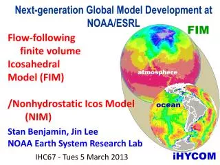
FIM basics. Rainer Bleck , Shan Sun, Tanya Smirnova (and a host of other contributors too numerous to mention) NOAA Earth System Research Laboratory, Boulder, Colorado July 2012. FIM. short for FFFVIM. Flow-following. Finite-volume. Icosahedral.


FIM basics
E N D
Presentation Transcript
FIM basics Rainer Bleck, Shan Sun, Tanya Smirnova (and a host of other contributors too numerous to mention) NOAAEarth System Research Laboratory, Boulder, Colorado July 2012
FIM short for FFFVIM Flow-following Finite-volume Icosahedral
Overriding goal:add genetic diversity to atmo and oceanic dycores • Unique combination of two (not quite so unique) grid types: • Icosahedral horizontal grid • Adaptive (terrain-following/isentropic) vertical grid • Tradeoffs: • Some drawbacks in traditional grids are avoided • must learn to cope with a few new problems
Horizontal grid: Pros and Cons • Pros: • No pole problems • Fairly uniform mesh size & cell shape on sphere • Cons: • Indirect addressing (an efficiency issue) • Wavenumber 5 zonal grid irregularity • Line-integral based discretizations hard to manipulate • Minor annoyances: • Model diagnostics, graphics display more complex
Adaptive vertical grid(primarily isentropic) Coordinate surfaces and isotachs: solid. Pot.temperature: color
How we maintain the vertical grid: Continuity Equation in generalized (“s”) coordinates (zero in fixedgrids) (zero in material coord.) (known)
Vertical grid: Pros and Cons • Pros (in q domain): • Numerical dispersion acts along isentropes • Optimal resolution of fronts and associated shear zones • Cons (in q domain): • Poor resolution in unstratifiedcolumns • Positive side effect of hybrid design: • Weak stratification due to surface heating leads to deep sigma domain (=> more uniform grid spacing at low latitudes)
FIM • Hydrostatic; primitive eqns (solved explicitly) • Arakawa A-grid (i.e. no staggering) • 3-level Adams-Bashforth time differencing • Finite-volume discretization; no explicit mixing terms required to suppress grid-scale noise • Variable vertical grid spacing requires transport eqns in flux form for conservation • Use FCT for pos-definiteness, monotonicity • Divergence, vorticity, gradients expressed as line integrals along grid cell perimeter • GFS column physics • Horiz/vert. resolution specified at runtime • highest resolution regularly used: ~15km (2.6M cells)
Seehttp://fim.noaa.govfor FIM documentation, skill scores, and twice-daily 10-day forecasts based on GFS initial conditions