Dielectrics
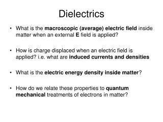
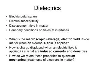
Dielectrics. Electric polarisation Electric susceptibility Displacement field in matter Boundary conditions on fields at interfaces What is the macroscopic (average) electric field inside matter when an external E field is applied ?

Dielectrics
E N D
Presentation Transcript
Dielectrics • Electric polarisation • Electric susceptibility • Displacement field in matter • Boundary conditions on fields at interfaces • What is the macroscopic (average) electric field inside matter when an external E field is applied? • How is charge displaced when an electric field is applied? i.e. what are induced currents and densities • How do we relate these properties to quantum mechanical treatments of electrons in matter?
Electric Polarisation Microscopic viewpoint Atomic polarisation in E field Change in charge density when field is applied r(r) Electronic charge density E No E field E field on Dr(r) Change in electronic charge density Note dipolar character r - +
Electric Polarisation Dipole Moments of Atoms Total electronic charge per atom Z = atomic number Total nuclear charge per atom Centre of mass of electric or nuclear charge Dipole moment p = Zea
E E E p P P + - Electric Polarisation Uniform Polarisation • Polarisation P, dipole moment p per unit volume Cm/m3 = Cm-2 • Mesoscopic averaging: P is a constant field for uniformlypolarisedmedium • Macroscopic charges are induced with areal density spCm-2
s- s+ E P s- s- Electric Polarisation • Contrast charged metal plate to polarised dielectric • Polarised dielectric: fields due to surface charges reinforce inside the dielectric and cancel outside • Charged conductor: fields due to surface charges cancel inside the metal and reinforce outside
E P s+ s- E- E+ Electric Polarisation • Apply Gauss’ Law to right and left ends of polarised dielectric • EDep = ‘Depolarising field’ • Macroscopic electric field EMac= E + EDep = E - P/o E+2dA = s+dA/o E+ = s+/2o E- = s-/2o EDep= E+ + E- = (s++ s-)/2o EDep= -P/o P = s+ = s-
E + - + - P + - Electric Polarisation Non-uniform Polarisation • Uniform polarisation induced surface charges only • Non-uniform polarisation induced bulk charges also Displacements of positive charges Accumulated charges
Electric Polarisation Polarisation charge density Charge entering xz face at y = 0: Py=0DxDz Cm-2 m2 = C Charge leaving xz face at y = Dy: Py=DyDxDz = (Py=0 + ∂Py/∂yDy) DxDz Net charge entering cube via xz faces: (Py=0 -Py=Dy)DxDz = -∂Py/∂yDxDyDz z Charge entering cube via all faces: -(∂Px/∂x + ∂Py/∂y + ∂Pz/∂z)DxDyDz = Qpol rpol= lim (DxDyDz)→0Qpol/(DxDyDz) -. P = rpol Dz Py=0 Py=Dy y Dy Dx x
Electric Polarisation Differentiate -.P = rpol wrt time .∂P/∂t + ∂rpol/∂t = 0 Compare to continuity equation .j + ∂r/∂t = 0 ∂P/∂t = jpol Rate of change of polarisation is the polarisation-current density Suppose that charges in matter can be divided into ‘bound’ or polarisation and ‘free’ or conduction charges rtot = rpol + rfree
Dielectric Susceptibility Dielectric susceptibility c (dimensionless) defined through P = ocEMac EMac = E– P/o oE = oEMac + P oE = oEMac + ocEMac= o (1 + c)EMac= oEMac Define dielectric constant (relative permittivity) = 1 + c EMac = E/ E = eEMac Typicalstatic values (w = 0) for e: silicon 11.4, diamond 5.6, vacuum 1 Metal: e → Insulator: e (electronic part) small, ~5, lattice part up to 20
Mion k melectron kMion Si ion Bound electron pair Dielectric Susceptibility Bound charges All valence electrons in insulators (materials with a ‘band gap’) Bound valence electrons in metals or semiconductors (band gap absent/small ) Free charges Conduction electrons in metals or semiconductors Resonance frequency wo ~ (k/M)1/2 or ~ (k/m)1/2 Ions: heavy, resonance in infra-red ~1013Hz Bound electrons: light, resonance in visible ~1015Hz Free electrons: no restoring force, no resonance
Mion k melectron kMion Dielectric Susceptibility Bound charges Resonance model for uncoupled electron pairs
Mion k melectron kMion Dielectric Susceptibility Bound charges In and out of phase components of x(t) relative to Eo cos(wt) in phase out of phase
Dielectric Susceptibility Bound charges Connection to c and e e(w) Im{e(w)} w = wo w/wo Re{e(w)}
s(w) Re{e(w)} wo = 0 Drude ‘tail’ w Im{s(w)} Dielectric Susceptibility Free charges Let wo→ 0 in c and e jpol = ∂P/∂t
Displacement Field Rewrite EMac = E– P/o as oEMac + P = oE LHS contains only fields inside matter, RHS fields outside Displacement field, D D = oEMac + P = oEMac= oE Displacement field defined in terms of EMac(inside matter, relative permittivity e) and E (in vacuum, relative permittivity 1). Define D = oE where is the relative permittivity and E is the electric field This is one of two constitutive relations e contains the microscopic physics
Displacement Field Inside matter .E = .Emac = rtot/o= (rpol + rfree)/o Total (averaged) electric field is the macroscopic field -.P = rpol .(oE + P) = rfree .D = rfree Introduction of the displacement field, D, allows us to eliminate polarisation charges from any calculation
Validity of expressions • Always valid: Gauss’ Law for E, P and D relation D =eoE + P • Limited validity: Expressions involving e and • Have assumed that is a simple number: P = eo E only true in LIH media: • Linear: independent of magnitude of E interesting media “non-linear”: P = eoE + 2eoEE + …. • Isotropic: independent of direction of E interesting media “anisotropic”: is a tensor (generates vector) • Homogeneous: uniform medium (spatially varying e)
Boundary conditions on D and E D and E fields at matter/vacuum interface matter vacuum DL = oLEL= oEL+PL DR = oRER= oERR=1 No free charges hence .D = 0 Dy = Dz = 0 ∂Dx/∂x = 0 everywhere DxL = oLExL= DxR = oExR ExL=ExR/L DxL= DxR E discontinuous D continuous
DR = oRER dSL qR qL dSR DL = oLEL Boundary conditions on D and E Non-normal D and E fields at matter/vacuum interface .D = rfreeDifferential form∫ D.dS = sfree, enclosed Integral form ∫ D.dS = 0 No free charges at interface -DL cosqL dSL + DR cosqR dSR = 0 DL cosqL = DR cosqR D┴L = D┴R No interface free charges D┴L - D┴R = sfree Interface free charges
ER dℓL qR qL dℓR EL Boundary conditions on D and E Non-normal D and E fields at matter/vacuum interface Boundary conditions on Efrom∫ E.dℓ = 0(Electrostatic fields) EL.dℓL + ER.dℓR = 0 -ELsinqLdℓL + ERsinqR dℓR = 0 ELsinqL = ERsinqR E||L = E||R E|| continuous D┴L = D┴R No interface free charges D┴L - D┴R = sfree Interface free charges
DR = oRER dSL qR qL dSR DL = oLEL Boundary conditions on D and E