Understanding Value-at-Risk (VaR) in Financial Risk Management
420 likes | 533 Views
Learn about VaR, a key risk measure for financial portfolios, and its role in quantifying market risk. Explore volatility estimation methods and the importance of correlations in risk assessment.

Understanding Value-at-Risk (VaR) in Financial Risk Management
E N D
Presentation Transcript
Chapter 20. Value-at-Risk (VaR) I. Motivation: A. Option sensitivities like delta, gamma, vega, ... , describe different aspects of risk for a portfolio. 1. Banks typically compute each of these measures every day for each of the market variables they are exposed to. Traders & managers for the firm must know their situation. 2. There may be hundreds of these market variables. This analysis leads to huge number of risk measures each day. -- too much information for senior management to use.
I.B. Definition of VaR 1. VaR is an attempt to provide a single number that summarizes the total risk in a portfolio of financial assets. 2. VaR aims to make a statement of the following form: “We are X% certain that we will not lose more than V dollars in the next N days.” 3. Appeal: easy to understand. Simply asks, how bad can things get? 4. The variable, V, is the VaR of the portfolio. V is a function of two parameters: N, the time horizon; X, the confidence level.
I.C. Regulators Require VaR for Banks 1. Calculation of VaR was made easier in Oct. 1994, when J.P. Morgan made its RiskMetrics database of volatilities and correlations freely available to all market participants. 2. The REGULATORS require Financial Institutions to use VaR. e.g., Banks are now required to calculate VaR; Regulators use VaR in determining required capital for a bank, to reflect the market risk it is bearing. 3. Bank regulators use N=10 and X=99; They consider losses over a 10-day period that are expected only 1% of the time.
I.D. Background for VaR Facts about the Normal distribution:
II. Volatilities A. The risk that a portfolio will lose value depends on the volatilities of the market variables it is exposed to. These volatilities play a key role in determining VaR. B. Definition. 1. Recall definition of volatility for B / S model: σ = stddevof continuously compounded return in ONE YEAR. T ½ = stddev of continuously compounded return earned in time T. ** The “Square Root Effect”: uncertainty increases as a function of sqrt(T). 2. In VaR calculations, T is measured in DAYS, so σ is "volatility per day." σday= stddev of continuously compounded return in ONE DAY, = stddev of proportional change in asset pricein ONE DAY. a. Note: σdayσyear / (252) ½ ; there are 252 trading days in one year. Thus, σdayσyear (.06).
II.C. Estimating Volatility 1. Define σn = volatility per day ( σday) for market variable, calculated on day n. Thus, σn2 = variance rate of the market variable on day n. 2. Standard approach: Estimate HISTORICAL VOLATILITY. Let { S1, S2, ..., Sn} be daily closing prices. Let ui= ln(Si / Si-1 ) = daily returns. Then σn2 = 1 / (n-1) Σ (ui - mean(u))2 Or, use approximation: Let mean(u) = 0; then σn2 = 1/n Σui2. [ Mean daily return ≈ 0; This is simple, & gives good approximation. ]
II.C. Estimating Volatility 3. Alternative approach: EWMA (Exponentially Weighted Moving Avg). a. The sample variance in 2. weights all ui2 terms equally (same weight on day 1 or day n). EWMA weights ui2 terms less if they are further back in time. Result: σn2= λ σn-12 + (1 - λ) un2 (0 < λ < 1). b. Note1: If you substitute successively for σn-12, σn-22, ... , you can see that σn2 depends on sum of past ui2 terms, where weights decline exponentially: 1st: Result is also true in period n-1: --- σn-12= λ σn-22 + (1-λ)un-12. Thus: σn2 = λ (λσn-22 + (1-λ)un-12) + (1-λ) un2= λ2 σn-22 + (1-λ)[λ un-12 + un2 ]. 2nd: Result is also true in period n-2: --- σn-22 = λ σn-32 + (1-λ)un-22. Thus: σn2 = λ2 (λσn-32 + (1-λ)un-22) + (1-λ) [λ un-12 + un2 ] = λ3 σn-32 + (1-λ)[λ2 un-22 + λ un-12 + un2 ]. kth: After k such substitutions, λk ≈ 0, so we get: σn2= λkσn-k2 + (1-λ)[un2 + λun-1 + λ2 un-22 + … + λk un-k2 ] or σn2 ≈ 0 + (1-λ)[un2 + λun-1 + λ2 un-22 + … + λk un-k2 + … ].
II.C. Estimating Volatility More on EWMA: n2 = n-12 + (1-) un2 3.c. Example: Let λ = .9, σn-1 = .01, and un = .02; Thenσn2= (.9)(.0001) + (.1)(.0004) = .00013 andσn= .0114 Note: In this example, return on day n (un = .02) > σn-1(= .01). Thus, when we add un2 to get our new estimate, this increases σn. If, instead, un < σn-1, this would decrease σn. Thus, updated estimates of σn depend greatly on recent un. Note1: EWMA approach can be updated easily each day. Simply keep current estimate of σn-1, & consider the new daily return, un. Note2: EWMA approach succeeds in tracking changes in volatility; If true σn2 ↑ over time, the values for ui2 will also ↑, so σn2will ↑. Note3: λ determines how responsive σn2 is to changes in ui2. Low value of λ means ui2terms further back mean less; recent ui2 more. High value of λ means ui2terms further back mean more; recent ui2 less.
III. Correlations A. Intuition: The risk that a portfolio will lose value also depends on the correlations among the market variables it is exposed to. 1. Suppose portfolio is exposed to risk that both Euro & Yen will ↓. We should consider whether these exchange rates are correlated! i.e., If Euro ↓, does Yen also tend to ↓? B. Definition. 1. Consider two market variables, U & V (returns/changes in 2 prices). Let: σu,n = daily volatility of variable U, calculated on day n; σv,n = daily volatility of variable V, calculated on day n; covn = covariance between daily returns, U & V, on day n. Then ρuv= covn / σu,nσv,n.
III.C. Estimating Correlations 1. Historical correlation measures -- equally weighted ui and vi: Let mean(u) = mean(v) = 0; Then: σu,n2 = 1/n Σ ui2 ; σv,n2= 1/n Σ vi2; covn= 1/n Σ uivi . Note: This formula gives equal weights to all uivi terms in covn. 2. EWMA: covn = λ covn-1+ (1-λ) un vn. Note: Weights on uiviterms decline as we move back in time. The lower the value of λ, the less weight on older terms, and the more weight is placed on recent observations. Note: Must be consistent how you treat σu,n2, σv,n2, and covn. If you get σu,n2 & σv,n2with equal (declining) weights, must also get covnwith equal (declining) weights.
IV. Simple Example A. Portfolio 1 consists of $10,000,000 in IBM stock (U); Daily Volatility = σu,n = .02 (corresponds to annual Vol of .02(252)½ = .32); Compute the VaR of this portfolio. Let N = 10 days, X = 99. Std Dev of change in IBM pfover 1 day = $10,000,000 (.02) = $200,000. Std Dev of change in IBM pfover 10 days = $10,000,000 (.02) (10½) = $200,000 (10½) = $632,456. Assume1: mean(U) = 0. This expected return is likely small relative to Std Dev. e.g., if E(r) over 1 year = 18%, then E(r) over 1 day = 18% / 252 = .07% [ much < 1-day σu,n = 2% ]; Assume2: U is normally distributed (i.e., S is lognormal). Then there is 99% chance S will not decrease more than 2.33 std dev. (Or a 95% chance S will not decrease more than 1.65 stddev). THUS, the 99% / 10-day VaRis 2.33 x $632,456 = $1,473,621; Or, the 95% / 10-day VaRis 1.65 x $632,456 = $1,043,552. 99% sure won’t lose > $1,473,621 in 10 days; 95% sure won’t lose > $1,043,552 in 10 days.
IV. Simple Example B. Portfolio 2 consists of $5,000,000 of AT&T stock (V); Daily Volatility = σv,n = .01 (corresponds to annual Volof .01(252)½ = .16); Std Dev of change in AT&T pfover 10 days = $5,000,000 x .01 x (10 ½) = $158,144 The 99% / 10-day VaRfor this portfolio is: 2.33 x $158,144 = $368,405; The 95% / 10-day VaRfor this portfolio is: 1.65 x $158,144 = $260,937. [ Less Value-at-Risk than Portfolio 1! ] C. Portfolio3 = Portfolio1 + Portfolio2. In addition, suppose we know ρuv = .7 We need the Std Dev of this portfolio, U + V. In general, σ(U + V) = [σU2+ σV2 + 2 ρ σUσV]½ For this example, we have σU = $632,456, and σV = $158,114. Thus, σ(U+V) = [$632,4562+ $158,1142+ 2(.7)(632,456)(158,144)]½ = $751,665 Then: 99% / 10-day VaRfor Portfolio3 is 2.33 x $751,665 = $1,751,379 Or: 95% / 10-day VaRfor Portfolio3 is 1.65 x $751,665 = $1,240,247
IV. Simple Example D. The Benefits of Diversification. If changes in value of IBM & AT&T were perfectly correlated (ρ = 1), VaR of Portfolio3 would be sum of VaR's of Portfolio's 1 & 2. If IBM and AT&T have correlation < 1, (ρ < 1), VaR of Portfolio3 will be < sum of VaR's of Portfolio's 1 & 2. HERE, ρ = .7; VaR for Portfolio1 (U) = $1,473,621; VaR for Portfolio2 (V) = $368,405; VaR for Portfolio3 (U + V) = $1,751,379. Benefits of Diversification = [ VaR(U) + VaR(V) ] - VaR(U+V) = [ $1,473,621 + $368,405 ] - $1,751,379 = $90,647 This exercise shows that lower correlation means lower VaR.
V. Linear Model A. VaR calculations are straightforward when (like in above example): 1. We assume that change in value of portfolio is linearly related to the changes in values of underlying market variables; 2. The changes in values of underlying market variables are normal. B. General Linear Model (GLM): Assume there are n underlying market variables; n ΔP = Σ αiΔxi i=1 where ΔP = $-change in portfolio value in one day; Δxi= prop. change (return) on underlying ith market variable during day; αi = constants. Define: σi = daily volatility of Δxi; ρij= correlation between Δxi and Δxj. n Then σp = daily volatility of ΔP, where σP2 = Σ αi2 σi2 + 2 Σ Σαiαjσiσjρij. i=1 i<j
V.B. General Linear Model 1. Redo previous example; n = 2 assets in Portfolio3; Δx1 & Δx2 are prop. changes in prices of IBM & AT&T in 1 day; Measuring values in millions of $, ΔP = 10Δx1 + 5Δx2[α1 = 10; α2 = 5] Also given: σ1 = .02; σ2 = .01; ρ12 = .7; Then σP2 = 102 x .022 + 52 x .012 + 2 x 10 x 5 x .02 x .01 x .7 = .0565 and σP = .238 = stddev of change in portfolio value per day; Then σP(10) ½ = .238 (10) ½ = .752 = std. dev. of ΔP over 10 days, and 99% / 10-day VaR= 2.33 x .752 = $1.751 million (same answer).
V.C. When Linear Model can be Used 1. When the payoff patterns of the assets in the portfolio are linear. a. Examples: i. Portfolio with no derivatives (stocks, bonds, foreign exchange, & commodities). Here ΔP is linearly dependent on the Δxi(changes in the underlying prices). ii. Portfolio with certain derivatives having linear payoff patterns. e.g.1 Forward contract to buy foreign currency maturing at T. This can be regarded as exchange of a foreign zero-coupon bond for a domestic zero-coupon bond, both maturing at time T. Therefore, we can rewrite this portfolio as linear combination of positions in bonds and foreign exchange, as in i., and ΔP depends linearly on zero-coupon bond prices and exchange rates. e.g.2 Interest rate SWAP. This can be regarded as exchange of a floating rate bond for a fixed rate bond. The fixed rate bond can be regarded as a portfolio of zero-coupon bonds. The floating rate bond will be worth par just after next payment. Thus the interest rate SWAP reduces to a portfolio of long and short positions in zero-coupon bonds.
V.D. Options have Nonlinear Payoffs Thus, linear model only holds approximately when portfolio contains options. 1. Explanation: Consider portfolio of options on a single stock. δ = ΔP / ΔS; or ΔP = δ ΔS where ΔS is the $ change in the stock price in 1 day. Define Δx as the proportional change (return) in the stock price in 1 day: Δx= ΔS / S; or S = S x Then an approximate relationship between ΔP and Δx is: ΔP = δ ΔS; or ΔP = S x = S x. When we have position in several market variables that includes options, we can derive approximately linear relation between ΔP & Δxi's similarly: n ΔP = Σ Si δiΔxi; where Si= price of ith market variable; i=1 and δi= delta of pfwrtithmkt variable. n This corresponds to old GLM equation: ΔP = Σ αiΔxi with αi= Si δi. i=1
V.D. Options have Nonlinear Payoffs 2. Example. Consider portfolio of options on IBM and AT&T. Let δ1= 1,000 = delta of IBM option position; = (∆P1 / ∆S1) δ2= 20,000 = delta of AT&T option position; = (∆P2 / ∆S2) S1= $120 = share price of IBM; S2= $30 = share price of AT&T; σ1= .02 = volatility of IBM price changes in one day; σ2= .01 = volatility of AT&T price changes in one day. (S1) (1) (S2) (2) As an approximation: ΔP = 120 x 1,000 Δx1+ 30 x 20,000 Δx2 or ΔP = 120,000 Δx1+ 600,000 Δx2 where Δx1 & Δx2 are prop. changes in prices of IBM & AT&T in 1 day, and ΔP is the resulting change in the portfolio. Then the Std Dev of ΔP in one day (in thousands of $) is: [ (120 x .02)2 + (600x.01)2 + 2 x 120 x .02 x 600 x .01 x .7 ] ½ = 7.689 Thus the 95% / 5-day VaRis: 1.65 x (5) ½ x 7,869 = $29,033.
VI. Quadratic Model Motivation: When Portfolio includes options, the linear model is only an approximation -- it ignores gamma, or curvature. A. Impact of gamma () on the probability distribution of ΔP. (Fig. 20.3 on top; Fig. 20.4, 20.5 on bottom.) 1. When > 0 (long options) distribskewed right. When < 0 (short options) distribskewed left. a. Payoff pattern on long call option ( > 0). If underlying market variable is normal, implied distribution is skewed to right. b. Payoff pattern on short call option ( < 0). If underlying market variable is normal, implied distribution is skewed to left.
VI. Quadratic Model Translation of Asset Price Change to Price Change for Long Call
VI. Quadratic Model Translation of Asset Price Change to Price Change for Short Call
VI.B. VaR of Portfolio depends on Left Tail for ΔP 99% VaR is value below which is only 1% of distribution (left tail). 95% VaR is value below which is only 5% of distribution (left tail). 1. Positive gamma portfolio is skewed to right; Has thin left tail & fat right tail (less downside). Thus, if you assume distribution of ΔP is normal, VaRtoo large; true left tail thinner than normal; Area under thin left tail is less than that under normal; so normalVaR suggests bigger loss than reality; should go less far left. 2. Negative gamma portfolio is skewed to left; Has fat left tail & thin right tail (more downside). Thus, if you assume distribution of ΔP is normal, VaRtoo small; true left tail fatter than normal; Area under fat left tail is more than that under normal; so normalVaR suggests smaller loss than reality; should go farther left.
VI.C. Better Estimation of VaR: Include both δ & 1. Consider a portfolio dependent on a single asset with price S. a. With Linear Model we assumed: δ = ΔP/ΔS; or ΔP = δ ΔS where ΔS is the $ change in the stock price in one day. b. More accurate relation: ΔP = δ ΔS + 1/2 ΔS2 (Taylor Series Exp.) c. Defining Δx as proportionate ∆Sin one day: Δx= ΔS / S, or ΔS = S Δx. d. We can substitute for ΔS above (in b.) to get: ΔP = S δ Δx + 1/2 S2Δx2 i. For portfolio with n underlying market variables, this becomes: (**1) ΔP = Σ Si δiΔxi+ Σ 1/2 Si2iΔxi2 where Si is ith market variable, and δi & iare its delta & gamma. ii. This equation generalizes to: (**2) ΔP = Σ αiΔxi + Σ βi Δxi2 where αi = Si δi and βi= 1/2 Si2i NOTE: Relation in i & ii is nonlinear in Δxi. Also, this assumes each option depends on only 1 mkt variable. Without this assumption, relation is more general: ΔP = Σ αiΔxi+ Σ Σ βijΔxi Δxj.
VI.C. Better Estimation of VaR: Include both δ & 2. Problem: This nonlinear model is not as easy to work with. Can be used with Simulation Approach (more later). a. Nonlinear Equation (**2) can be used to calculate moments for ΔP: n E(ΔP) = Σ βiσi2 ; since E(Δxi) = 0; i=1 n n E(ΔP2) = Σ Σ[ αiαjσiσjρij+ βiβj σi2 σj2(1 + 2 ρij2 ) ] i=1 j=1 b. These moments can be fitted to a normal distribution. (However, once again, assumption of normality is not great.) c. Can also calculate higher moments of ΔP (skewness, kurtosis). Higher moments can then be used with the Cornish-Fisher expansion to estimate the fractilesof the probability distribution of ΔP that correspond to any required VaR.
VII. Monte Carlo Simulation A. Alternative approach: Use Simulation to get probability distrib. for ΔP. To calculate a one-day VaR for a portfolio: 1. Value the portfolio today, using current values of market variables. 2. Sample once from multivariate normal probability distrib. of Δxi's. (Pick parameters -- moments -- of distrib. as desired. See VI.C.2.) 3. Use values of Δxi'sthat are sampled to determine simulated new value of each market variable at end of the day. 4. Revalue portfolio at end of the day using the new sampled values. 5. Subtract value in step 1 from that in step 4 to get sample ΔP. 6. Repeat steps 2 - 5 many times to build probability distrib. for ΔP.
VII. Monte Carlo Simulation B. VaR is computed as proper fractile of probability distrib. of ΔP. 1. For example, calculate 5,000 sample values for ΔP. The 99% / 1-day VaRis value of ΔP for 50th worst outcome; The 95% / 1-day VaRis value of ΔP for 250th worst outcome; … The N-day VaRis then calculated as the 1-day VaR times (N)½ . 2. Drawback of simulation -- computationally intensive (no problem!). A company's complete portfolio (maybe thousands of assets) has to be revalued many times (step 4). a. Can speed procedure by assuming that equation (**2) describes the relation between ΔP and the Δxi's. (Can then skip steps 3 & 4 each iteration; no need to revalue the portfolio every time.)
VIII. Use of Historical Data A. Can calculate VaR from simulation based on historicalmkt behavior. 1. First create a database consisting of daily movements in all market variables over several years. 2. The first simulation trial lets the % changes in all market variables be those experienced on the first day in the database. 3. The second simulation ... on the second day. And so on. 4. The change in portfolio, ΔP, is calculated for each simulation trial and VaR is calculated as proper fractile of the prob. distrib. of ΔP. Here the change in portfolio value can be obtained either by revaluing, or by using equation (**2).
VIII. Use of Historical Data B. Advantage: This accurately reflects historicaldistrib. of mkt variables. C. Disadvantages: 1. Number of simulation trials is limited to number of days in database. 2. Sensitivity analyses are difficult. (With statistical simulation, can change distrib. parameters & rerun.) 3. Variables for which there are no mktdata cannot easily be included. D. Kurtosis. 1. For many mktvariables, the probability distrib of the Δxi and ΔP that is calculated from historical data often exhibits fat tails, so that extreme outcomes are more likely than normal distrib.. This is positive kurtosis. This can be modeled in the simulation ...
IX. Stress Testing A. Can examine how current portfolio would perform under the most extreme market moves seen in the last 10 to 20 years. 1. To test impact of extreme movement in U.S. stock market: a. Could let prop. change in all market variables (Δxi's) equal those on Oct. 19, 1987 (when S&P 500 changed 22.3 stddev’s). b. Could use Δxi's on Jan. 8, 1988 (S&P 500 changed 6.8 σ's). 2. To test impact of extreme movement in U.K. interest rates: a. Could use Δxi'son Apr 10, 1992 (10-yr bond yield rose 7.7 σ's).
IX. Stress Testing B. A way to consider implications of extreme events that happen, but are almost impossible according to normalprob. distribution. 1. For example, under normal distribution, a change of 5σ's happens one day every 7,000 years. In practice, we have seen this once or twice every 10 or so years. C. Simple to do. Once we have the variance of the in value of the portfolio over 1-day, we can multiply this by any number of standard deviations desired, and then multiply by (N)½ to get N-day VaR at any confidence level.