Two Methods of Localization Model Covariance Matrix Localization (B Localization)

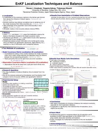
1. EnKF Localization Techniques and Balance 1Steven J. Greybush, 1Eugenia Kalnay, 2Takemasa Miyoshi 1University of Maryland, College Park, MD, U.S.A. 2Numerical Prediction Division, Japan Meteorological Agency, Tokyo, Japan • Results from Assimilation of Gridded Observations • Assimilate 20 observations of h and v (randomly perturbed from the truth) at regular intervals along the domain; observe accuracy and balance of the analysis. • Localization • A modification of the covariance matrices in the Kalman gain formula that reduces the influence of distant regions. (Houtekamer and Mitchell, 2001) • Removes spurious long distance correlations due to sampling error of the model covariance from finite ensemble size. (Anderson, 2007) • Takes advantage of the ensemble's lower dimensionality in local regions. (Hunt et. al., 2007) • Ultimately creates a more accurate analysis (reduces RMSE). Localization Distance L=1000 km; Distance between Observations D = 500 km; Wavelength W = 2000 km Analysis Increments: Initial Waveforms: • Balance • Lorenc (2003) and Kepert (2006) argue that localization reduces the balance information encoded in the model covariance matrix. • Houtekamer and Mitchell (2005) noted balance issues when applying a localized EnKF to the Canadian GCM. • Imbalanced analyses project information onto inertial-gravity waves, which are filtered out (geostrophic adjustment, digital filtering, etc.), resulting in a loss of information and a suboptimal analysis. • Two Methods of Localization • Model Covariance Matrix Localization (B Localization) • Accomplished by taking a Schur product between the model covariance matrix and a matrix whose elements are dependent upon the distance between the corresponding grid points. (Hamill et al., 2001) • Model grid points that are far apart have zero error covariance. • Observation Covariance Matrix Localization (R Localization) • Observations that are far away from a grid point have infinite error. K = BHT(HBHT + R)-1 Analysis Imbalance: B Localization >> R Localization > No Localization Analysis RMS Error: B Localization < R Localization < No Localization • Results from Monte Carlo Simulations • Three scales in the problem: W = wavelength of solutions L = localization distance D = distance between observations • Explore the phase space of the three scales. • Obtain robust results by repeating each scenario 100x with random observation errors. L Bloc = B * exp(-(ri-rj)2 / 2L2) Rloc = R * exp(+(d)2 / 2L2) Constant D=500 km, W=2000 km, vary L: • Research Questions • How does localization introduce imbalance into an analysis? Can it be avoided? • How do the analyses produced by B-localization and R-localization EnKF compare in terms of accuracy (RMSE) and (geostrophic) balance? • Experimental Setup • Model • The shallow water equations in a rotating, inviscid fluid. • Variation only along the x-axis. • The variables of interest are h and v. • Linearize the equations, and apply a harmonic form to the solution. • Substituting into the governing equations, and assuming geostrophic balance, yields the following solutions for h and v: • Ensemble • Initially geostrophic waveform for truth and 2 ensemble members. • 101 Grid Points every 50 km along domain. Constant D=250 km, vary L and W: (warmer colors show greater imbalance) • Use ageostrophic wind as measure of imbalance. • vageo = v – g/f dh/dx • Localize the waveforms with L=1500 km. • |-dh/dx| increases while |v| decreases, disrupting the balance between the wind field and the mass field. (Lorenc 2003) Initial Ensemble and Truth • Conclusions • Both types of localization do introduce imbalance into analysis increments, especially for short localization distances. • R localization is significantly more balanced than B localization, but is slightly less accurate. • Future Work • Complement this study by comparing balance for B localization and R localization EnSQRT data assimilation on the SPEEDY GCM (Molteni, 2003), using realistic observation densities and locations. • Further investigate the mathematical properties of the two localization methods. Imbalance (Ageostrophic Wind) Localized Ensemble • Acknowledgements • Thanks to Kayo Ide and Jeff Anderson for their helpful comments and critiques of this project. WCRP/THORPEX WORKSHOP on 4D-VAR and ENSEMBLE KALMAN FILTER COMPARISONSBuenos Aires, Argentina; November 10-13, 2008