Download
1 / 39
440 likes | 820 Views
Data Structures – LECTURE 16 All shortest paths algorithms. Properties of all shortest paths Simple algorithm: O (| V | 4 ) time Better algorithm: O (| V | 3 lg | V |) time Floyd-Warshall algorithm: O (| V | 3 ) time Chapter 25 in the textbook (pp 620–635). All shortest paths.

E N D
Data Structures – LECTURE 16 All shortest paths algorithms • Properties of all shortest paths • Simple algorithm: O(|V|4) time • Better algorithm: O(|V|3 lg |V|) time • Floyd-Warshall algorithm: O(|V|3) time Chapter 25 in the textbook (pp 620–635).
All shortest paths • Generalization of the single source shortest-path problem. • Simple solution: run the shortest path algorithm for each vertex complexity is O(|E|.|V|.|V|) = O(|V|4) for Bellman-Ford and O(|E|.lg |V|.|V|) = O(|V|3 lg |V|) for Dijsktra. • Can we do better? Intuitively it would seem so, since there is a lot of repeated work exploit the optimal sub-path property. • We indeed can do better: O(|V|3).
2 3 1 5 4 All-shortest paths: example (1) 4 3 8 1 7 -5 2 -4 6
2 3 1 5 2 4 5 3 4 1 2 3 4 5 pred 1 2 3 4 5 dist All-shortest paths: example (2) 1 4 3 4 0 3 -3 8 8 1 1 7 1 7 -5 2 -5 -4 2 -4 6 6 -4 2
2 2 1 5 4 3 5 1 3 4 1 2 3 4 5 pred 1 2 3 4 5 dist All-shortest paths: example (3) 0 4 3 -4 4 3 3 8 8 1 1 7 7 -5 2 -5 -4 2 -4 6 6 -1 1
All shortest-paths: representation We will use matrices to represent the graph, the shortest path lengths, and the predecessor sub-graphs. • Edge matrix: entry (i,j) in adjacency matrix W is the weight of the edge between vertex i and vertex j. • Shortest-path lengths matrix: entry (i,j) in L is the shortest path length between vertex i and vertex j. • Predecessor matrix: entry (i,j) in Π is the predecessor of j on some shortest path from i (null when i = j or when there is no path).
All-shortest paths: definitions Edge matrix: entry (i,j) in adjacency matrix W is the weight of the edge between vertex i and vertex j. Shortest-paths graph: the graphs Gπ,i = (Vπ,i, Eπ,i) are the shortest-path graphs rooted at vertex I, where:
2 3 1 5 4 Example: edge matrix 1 2 3 4 5 4 1 2 3 4 5 3 8 1 7 -5 2 -4 6
2 3 1 5 4 Example: shortest-paths matrix 1 2 3 4 5 4 1 2 3 4 5 3 8 1 7 -5 2 -4 6
2 3 1 5 4 Example: predecessor matrix 1 2 3 4 5 4 3 1 2 3 4 5 8 1 7 -5 2 -4 6
The structure of a shortest path • All sub-paths of a shortest path are shortest paths. Let p = <v1, .. vk> be the shortest path from v1 to vk. The sub-path between vi and vj, where 1 ≤ i,j ≤ k,pij = <vi, .. vj> is a shortest path. • The shortest path from vertex i to vertex j with at most m edges is either: • the shortest path with at most (m-1) edges (no improvement) • the shortest path consisting of a shortest path within the (m-1) vertices + the weight of the edge from a vertex within the (m-1) vertices to an extra vertex m.
Recursive solution to all-shortest paths Let l(m)ij be the minimum weight of any path from vertex i to vertex j that has at most m edges. When m=0: For m≥ 1, l(m)ijis the minimum of l(m–1)ijand the shortest path going through the vertices neighbors:
All-shortest-paths: solution • Let W=(wij) be the edge weight matrix and L=(lij)the all-shortest shortest path matrix computed so far, both n×n. • Compute a series of matrices L(1), L(2), …, L(n–1) where for m = 1,…,n–1, L(m) = (l(m)ij) is the matrix with the all-shortest-path lengths with at most m edges.Initially, L(1) = W, and L(n–1) containts the actual shortest-paths. • Basic step: compute L(m) from L(m–1) and W.
Algorithm for extending all-shortest paths by one edge: from L(m-1) to L(m) Extend-Shortest-Paths(L=(lij),W) n rows[L] Let L’ =(l’ij) be an n×n matrix. fori 1 to ndo forj 1 to ndo l’ij ∞ fork 1 to ndo l’ij min(l’ij, lik + wkj) return L’ Complexity: Θ(|V|3)
This is exactly as matrix multiplication! Matrix-Multiply(A,B) n rows[A] Let C =(cij) be an n×n matrix. fori 1 to ndo forj 1 to ndo cij 0 (l’ij ∞) fork 1 to ndo cij cij+ aik.bkj(l’ij min(l’ij, lij + wkj)) return L’
2 1 4 3 5 4 3 8 1 7 -5 2 -4 6 Paths with at most two edges
2 1 4 3 5 4 3 8 1 7 -5 2 -4 6 Paths with at most three edges
2 1 4 3 5 4 3 8 1 7 -5 2 -4 6 Paths with at most four edges
2 1 4 3 5 4 3 8 1 7 -5 2 -4 6 Paths with at most five edges
All-shortest paths algorithm All-Shortest-Paths(W) n rows[W] L(1) W form 2 to n–1 do L(m) Extend-Shortest-Paths(L(m–1),W) return L(m) Complexity: Θ(|V|4)
Since the final product is equal to L(n–1) only |lg(n–1)| iterations are necessary! Improved all-shortest paths algorithm • The goal is to compute the final L(n–1), not all the L(m) • We can avoid computing most L(m) as follows: L(1) = W L(2) = W.W L(4) = W4 =W2.W2 … repeated squaring
Faster-all-shortest paths algorithm Faster-All-Shortest-Paths(W) n rows[W] L(1) W while m < n–1 do L(2m) Extend-Shortest-Paths(L(m),L(m)) m 2m return L(m) Complexity: Θ(|V|3 lg (|V|))
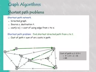
Floyd-Warshall algorithm • Assumes there are no negative-weight cycles. • Uses a different characterization of the structure of the shortest path. It exploits the properties of the intermediate vertices of the shortest path. • Runs in O(|V|3).
p k1 k2 i j Structure of the shortest path (1) • An intermediate vertexvi of a simple path p=<v1,..,vk> is any vertex other than v1 or vk. • Let V={1,2,…,n} and let K={1,2,…,k} be a subset for k≤ n. For any pair of vertices i,j in V, consider all paths fromi to j whose intermediate vertices are drawn from K. Let p be the minimum-weight path among them.
Structure of the shortest path (2) • k is not an intermediate vertex of path p: All vertices of path p are in the set {1,2,…,k–1} a shortest path from i to j with all intermediate vertices in {1,2,…,k–1} is also a shortest path with all intermediate vertices in {1,2,…,k}. 2.k is an intermediate vertex of path p: Break p into two pieces: p1 from i to k and p2 from k to j. Path p1 is a shortest path from i to k and path p2 is a shortest path from k to j with all intermediate vertices in{1,2,…,k–1}.
all intermediate vertices in{1,2,…,k–1} all intermediate vertices in{1,2,…,k–1} p1 p2 all intermediate vertices in{1,2,…,k} k j i Structure of the shortest path (3)
Recursive definition Let d(k)ij be the weight of a shortest path from vertex i to vertex j for which all intermediate vertices are in the set {1,2,…,k}. Then: The matrices D(k) = (d(k)ij) will keep the intermediate solutions.
4 3 5 Example: Floyd-Warshall algorithm (1) 2 4 3 8 1 1 7 -5 2 -4 6 K={1} Improvements: (4,2) and (4,5)
4 5 Example: Floyd-Warshall algorithm (2) 2 4 3 8 3 1 1 7 -5 2 -4 6 K={1,2} Improvements: (1,4) (3,4),(3,5)
5 Example: Floyd-Warshall algorithm (3) 2 4 3 8 3 1 1 7 -5 2 -4 4 6 K={1,2,3} Improvement: (4,2)
5 Example: Floyd-Warshall algorithm (4) 2 4 3 8 3 1 1 7 -5 2 -4 4 6 K={1,2,3,4} Improvements: (1,3),(1,4) (2,1), (2,3), (2,5) (3,1),(3,5), (5,1),(5,2),(5,3)
Example: Floyd-Warshall algorithm (5) 2 4 3 8 3 1 1 7 -5 2 -4 5 4 6 K={1,2,3,4,5} Improvements: (1,2),(1,3),(1,4)
Transitive closure (1) • Given a directed graph G=(V,E) with vertices V = {1,2,…,n} determine for every pair of vertices (i,j) if there is a path between them. • The transitive closure graph of G, G*=(V,E*) is such that E* = {(i,j): if there is a path i and j}. • Represent E* as a binary matrix and perform logical binary operations AND (/\) and OR (\/) instead of min and + in the Floyd-Warshall algorithm.
Transitive closure (2) The definition of the transitive closure is: The matrices T(k) indicate if there is a path with at most k edges between s and i.
Transitive closure algorithm Transitive-Closure(W) n rows[W] T(0) Binarize(W) fork 1 to ndo fori 1 to ndo forj 1 to ndo return T(n) Complexity: Θ(|V|3)
Summary • Adjacency matrix representation is the most convenient for representing all-shortest-paths. • Computing all shortest-paths is akin to taking the transitive closure of the edge weights. • Matrix multiplication algorithm runs inO(|V|3 lg |V|). • The Floyd-Warshall algorithm improves paths through intermediate vertices instead of working on individual edges. • Its running time: O(|V|3).
Other graph algorithms • Many more interesting problems, including network flow, graph isomorphism, coloring, partition, etc. • Problems can be classified by the type of solution. • Easy problems: polynomial-time solutions O(f (n)) where f (n) is a polynomial function of degree at most k. • Hard problems: exponential-time solutions O(f (n)) where f (n) is an exponential function, usually 2n.
Easy graph problems • Network flow – maximum flow problem • Maximum bipartite matching • Planarity testing and plane embedding.
Hard graph problems • Graph and sub-graph isomorphism. • Largest clique, Independent set • Vertex tour (Traveling Salesman problem) • Graph partition • Vertex coloring However, not all is lost! • Good heuristics that perform well in most cases • Polynomial-time approximation algorithms