Download
1 / 13
130 likes | 346 Views
Maximization of Production Output Subject to a Cost Constraint Appendix 6A. Max output (Q) subject to a cost constraint. Let C K be the cost of capital and C L the cost of labor Max L = Q - {C L •L + C K •K - C} L L : Q/ L - C L • = 0 MP L = C L

E N D
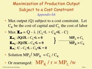
Maximization of Production Output Subject to a Cost ConstraintAppendix 6A • Max output (Q) subject to a cost constraint. Let CK be the cost of capital and CL the cost of labor • Max L = Q -{CL•L + CK•K - C} LL: Q/L - CL• = 0 MPL = CL LK: Q/K- CK• = 0 MPK = CK L: C - CL•L - CK•K = 0 • SolutionMPL/ MPK = CL / CK • Or rearranged: MPK / r = MPL /w } 2005 South-Western Publishing
Production Decisions and Linear ProgrammingAppendix 7B • Manufacturers have alternative production processes, some involving mostly labor, others using machinery more intensively. • The objective is to maximize output from these production processes, given constraintson the inputs available, such as plant capacity or union labor contract constraints. • A number of business problems haveinequality constraints, as in a machine cannot work more than 24 hours in a day. Linear programming works for these types of constraints
Using Linear Programming • Constraints of production capacity, time, money, raw materials, budget, space, and other restrictions on choices. • These constraints can be viewed as inequality constraints, or . • A "linear" programming problem assumes a linear objective function, and a series of linear inequality constraints
Linearity implies: 1. constant prices for outputs (as in a perfectly competitive market). 2. constant returns to scale for production processes. 3. Typically, each decision variable also has a non-negativity constraint. For example, the time spent using a machine cannot be negative.
Solution Methods • Linear programming problems can be solved using graphical techniques, SIMPLEX algorithms using matrices, or using software, such as Lindo or ForeProfit software*. • In the graphical technique, each inequality constraint is graphed as an equality constraint. The Feasible Solution Space is the area which satisfies all of the inequality constraints. • The Optimal Feasible Solution occurs along the boundary of the Feasible Solution Space, at the extreme points or corner points. *www.lindo.comor ForeProfit at : www.swlearning.com/economics/mcguigan/learning_resources.html
The corner point that maximize the objective function is the Optimal Feasible Solution. • There may be several optimal solutions. Examination of the slope of the objective function and the slopes of the constraints is useful in determining which is the optimal corner point. • One or more of the constraints may be slack, which means it is not binding. • Each constraint has an implicit price, the shadow price of the constraint. If a constraint is slack, its shadow price is zero. • Each shadow price has much the same meaning as a Lagrangian multiplier.
TWO DIMENSIONAL LINEAR PROGRAMMING Corner Points A, B, and C X1 CONSTRAINT # 1 A B Feasible Region Is OABC CONSTRAINT # 2 C O X2
X1 CONSTRAINT # 1 Greatest Output Optimal Feasible Solution at Point B A B CONSTRAINT # 2 C O X2
Process Rays: Figure 7B.3 P1 L • Each lamp is a different production process (a combination of labor & capital) • P1 requires 1 hour of capital and 4 hours of labor • P2 requires 2 hours of capital and 2 hours of work • P3 requires 5 hours of capital and 1 hour of work • Combinations of labor and capital produce lamps: Q1 + Q2 +Q3 • The shaded box is the constraint on time for L and K P2 B 8 P3 K 5
Maximization Problem There are three types of lamps produced each day. There are but 8 hours of labor available a day and There are only 5 hours of capital machine hours. Maximize Q1 + Q2 +Q3 subject to: Q1 + 2·Q2 + 5Q3<5 The capital constraint of 5 hours per day. 4Q1 + 2·Q2 + Q3<8 The labor constraint of 8 hours per day. where Q1, Q2 and Q3 > 0 Nonnegativity constraint.
Feasible Region • If all inputs were used in making process 1, which takes 4 hours of labor and 1 hour of machine time, we’d make 2 lamps, but have slack machine time. This is feasible, but not optimal. • At point B on Figure 7B.3, all inputs are used. It involves some of Process 1 and some of Process 2. • Using the two rays, Point B can be reached by creating a parallelogram of the two rays.
A Parallelogram of Process Rays P1 L • Using 4 hours of labor and 1 hour capital makes 1 using process P1 • Using the remaining 4 hours of labor and 4 hours of machine time makes 2 lamps using process P2. • Solution: 3 lamps (one of type 1 and 2 of type 2) P2 B 8 P3 K 5 Figure 7B.3
Complexity and theMethod of Solution • The solutions to linear programming problems may be solved graphically, so long as this involves two dimensions. • With many products, the solution involves the SIMPLEX algorithm, or software available in FOREPROFIT or LINDO.