Download
1 / 74
740 likes | 880 Views
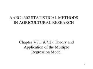
AAEC 4302 STATISTICAL METHODS IN AGRICULTURAL RESEARCH. Chapter 7(7.1 &7.2): Theory and Application of the Multiple Regression Model. Introduction. The multiple regression model aims to and must include all of the independent variables X1, X2, X3, …, Xk that are believed to affect Y

E N D
AAEC 4302 STATISTICAL METHODS IN AGRICULTURAL RESEARCH Chapter 7(7.1 &7.2): Theory and Application of the Multiple Regression Model
Introduction • The multiple regression model aims to and must include all of the independent variables X1, X2, X3, …, Xk that are believed to affect Y • Their values are taken as given: It is critical that, although X1, X2, X3, …, Xk are believed to affect Y, Y does not affect the values taken by them • The multiple linear regression model is given by: Yi = β0 + β1X1i + β2X2i + β3X3i +…+ βkXki + ui where i=1,…,n represents the observations, k is the total number of independent variables in the model, β0, β1,…, βk are the parameters to be estimated and ui is the disturbance term, with the same properties as in the simple regression model
The Model • In our example we have a time series data, k is five and i is twenty one. • The model to be estimated, therefore, is Yi = β0 + β1X1i + β2X2i + β3X3i +β4X4i + ui • As before: E[ Yi ]= β0 + β1X1i + β2X2i + β3X3i +…+ βkXki Yi = E[Yi]+ ui , the systematic (explainable) and unsystematic (random) components of Yi • And the corresponding prediction of Yi: Yi = β0 + β1X1i + β2X2i + β3X3i +β4X4i ^ ^ ^ ^ ^ ^
Model Estimation • Also as before, the parameters of the multiple regression model (βo, β1, β2, β3, β4) are estimated by minimizing SSR: SSR = ei2= (Yi-β0 - β1X1i - β2X2i - β3X3i - β4X4i )2 • As before, the formulas to estimate the regression model parameters that would make the SSR as small as possible n n ^ ^ ^ ^ ^ i=1 i=1
Y X2 Regression surface (plane) E[Y] = Bo+B1X1+B2X2 Ui X2 slope measured by B2 Bo X1 slope measured by B1 X1
Interpretation of the Coefficients ^ • The intercept βo estimates the value of Y when all of the independent variables in the model take a value of zero; which may not be empirically relevant or even correct in some cases. • In our example βo , is 144.94, which means that if : • Yi = 144.94+β1*(0)+β2*(0) + β3*(0)+β4*(0) • All the independent variables take the value of zero (price of beef is zero cents/lb, price of chicken is zero cents/lb, price of pork is zero cents/lb, and the income for US population is zero dollars/ per – year, then the estimated beef consumption will be 144.94 lbs/year). ^ ^ ^ ^ ^
Interpretation of the Coefficients ^ ^ ^ • In a strictly linear model, β1, β2,..., βk are slopes of coefficients that measure the unit change in Y when the corresponding X (X1, X2,..., Xk) changes by one unit and the values of all of the other independent variables remain constant at any given level (it does not matter which) • Ceteris paribus (other things being equal)
Interpretation of the Coefficients ^ • In our example: • β1= -0.00291. That means, if the price of beef increases by one cent/lb then the beef consumption will decrease by 0.00291 pounds per – year, ceteris paribus • β2= -0.116. That means, if the price of chicken increases by one cent/lb then the beef consumption will decrease by 0.116 pounds per – year, ceteris paribus (Does this result makes sense?) ^ ^
Interpretation of the Coefficients ^ • In our example: • β3= 0.3413. That means, if the price of pork increases by one cent/lb then the beef consumption will increase by 0.3413 pounds per – year, ceteris paribus (beef and pork are substitutes). • β4= 0.3121. That means, if the US income increases by one dollar per year then beef consumption will increase by 0.3121 pounds per – year, ceteris paribus ^ ^
The Model’s Goodness of Fit • The same key measure of goodness of fit is used in the case of the multiple regression model: R2 = 1 - { ei2/ (Yi-Y)2} • A disadvantage of the regular R2 as a measure of a model’s goodness of fit is that it always increases in value as independent variables are added into the model, even if those variables can’t be statistically shown to affect Y n n i=1 i=1
The Model’s Goodness of Fit • The adjusted or corrected R2 denoted by R2 is better measure to assess whether the adding of an independent variable likely increases the ability of the model to predict Y: R2 = 1 [{ei2/(n-k-1)}/{(Yi-Y)2/(n-1)}] • The R2 is always less than the R2, unless the R2 = 1 • Adjusted R2 lacks the same straightforward interpretation as the regular R2; under unusual circumstances, it can even be negative
The Specification Question • Any variable that is suspected to directly affect Y, and that did not hold a constant value throughout the sample, should be included in the model • Excluding such a variable would likely cause the estimates of the remaining parameters to be “incorrect”; i.e. the formulas for estimating those parameters would be biased • The consequences of including irrelevant variables in the model are less serious; if in doubt, this is preferred
AAEC 4302ADVANCED STATISTICAL METHODS IN AGRICULTURAL RESEARCH Chapters 6.3 Variables & Model Specifications
Lagged Variables • In many cases the value of Y in time period t is more likely explained by the value taken by X in the previous time period: For example, a farmer’s current year investment decisions might be based on the previous year prices, since the current year prices are not known when making these decisions.
Lagged Variables • In multiple regression models (i.e. models with more than one explanatory variable), it can be assumed that Y is affected by different lags of X:
Lagged Variables • The model can also be estimated using the OLS method (i.e. the previously developed formulas for calculating ( and ) • It is only necessary to rearrange the data in such a way that the value of Y at time period t coincides with the value of X at time period t-1
Lagged Variables Suppose we want to estimate cotton acres planted in the US (Y) as a function of the last 3 years price of cotton lint (Xt), cents/lb. What's the interpretation of: = 1.2 ? It means that if the price of cotton lint three years ago (t-3), changed by 1 cent per pound; the # of acres of planted cotton today (time, t) would increase by 1.2 acres, while holding all the other X’s constant.
First Differences of a Variable • The first difference of a variable is its change in value from one time period to the next • First difference on Y: • First difference on X: • The only reason you do this is if you believe that it is not the previous year that affects Yt; but the difference between the previous year and current year that affects Yt.
First Differences of a Variable Suppose you wanted to estimate the function where investment is a function of the change in GNP (i.e. first difference).
Examples of First Difference Models • In economics, the demand for durable goods could be more directly affected by the change in interest rates than by the interest rate level (a first difference in the independent variable) • In forestry, deforestation (i.e. the change in the forest cover from one year to the next) could be more directly related to the price of wood than total forest cover (a first difference in the dependent variable)
AAEC 4302ADVANCED STATISTICAL METHODS IN AGRICULTURAL RESEARCH Chapters 6.4-6.5, 7.4 Variables & Model Specifications
The Reciprocal Specification (6.4) • The reciprocal model specification is:
The Reciprocal Specification • Relationship between Y and the transformed independent variable is linear
The Reciprocal Specification • Model specified relation between inflation and unemployment as reciprocal, observations for 15 observations (1956-1970): • UINVi = 1/UMPLi • INFLi = B0 + B1*UINVi + ei • The estimated regression is: INFLi = -1.984+ 22.234*UINVi R2= 0.549 SER=0.956
The Reciprocal Specification • B0 =-1.984 • As UNEML increases, INFL decreases and approaches the lower limit of -1.984 percent • Quantitative implications are understood when we compare diff. predicted values of INFL for diff. rates of unemployment • If UNEMPL = 3%, INFL = -1.984 +22.234*(1/3) = 5.43 % • If UNEMPL = 4%, INFL = -1.984 +22.234*(1/4) = 3.57 %
The Log-Linear Specification (6.5) • A special type of non-linear relations become linear when they are transformed with logarithms • Specifically, consider • We take natural logs of both sides of this equation: • This is also known as the Log-Log or Double-Log specification, because it becomes a linear relation when taking the natural logarithm of both sides
The Log-Linear Specification • Also note that in a Log-Linear specification all ( and values must be positive, since the natural logarithm of a non-positive number is not defined • An important feature is that directly measures the elasticity of Y with respect to Xj; i.e. the percentage change in Y when Xj changes by one percent
The Log-Linear Specification • Model of aggregate demand for money in the US • Ln Mi= Bo + B1 ln GNPi + Ui • Estimated regression: LnMi= 3.948 + 0.215 LnGNPi R2 = 0.78 SER=0.0305
The Log-Linear Specification • B1= 0.215, or 0< B1<1 the elasticity of M with respect to GNP is 0.215 • 5% increase in GNP leads to 0.215*5=1.075% increase in predicted M • Predict demand for money when GNP = 1000: ln1000=6.908 lnM = 3.948 + 0.215*6.908 = 5.433 Antilog of 5.433 = 222.8 bill $
The Polynomial Specification (7.4) • A polynomial model specification (with respect to only) is: An advantage of the polynomial model specification is that it can combine situations in which some of the independent variables are non-linearly related to Y while others are linearly related to Y
The Polynomial Specification • A polynomial model can be estimated by OLS, viewing as any other independent variable in the multiple regression • In the example before j=1, i.e. a polynomial specification with respect to is desired: both ( and would be included as independent variables in the data set given to the Excel program for OLS (linear regression) estimation
The Polynomial Specification Multiple regression : Cross-sectional DB with 100 observations Estimated EANRS function: EANRSi = -9.791 +0.995 EDi + 0.471EXPi – 0.00751EXPSQi R2=0.329 SER4.267 B 1= 0.995 – holding the level of experience constant one additional year of education increases earnings by $995 EANRSi = constant + 0.471EXPi – 0.00751EXPSQi where the “constant” depends of the particular value chosen for ED
The Polynomial Specification • Slope = 0.471 + (2)(-0.00751)EXP • If EXP = 5 years, then slope = 0.471 + (2)(-0.00751)(5) = 0.396 thou $ A man with 5 years of experience will have his earnings increased by 396 $ after gaining one additional year of experience
Semi log Model Specification • Yi = β0 + β1 ln Xi + ui • ln Yi = β0 + β1 Xi + ui • ln Earngi = 0.673 + 0.107 Edui • One additional year of schooling increases earnings by the proportion of 0.107 or 10.7%
AAEC 4302ADVANCED STATISTICAL METHODS IN AGRICULTURAL RESEARCH Chapter 7.3 Dummy Variables
Use of Dummy Variables • In many models, one or more of the independent variables is qualitative or categorical in nature • This type of independent variables have to be modeled through dummy variables • A set of dummy variables is created for each categorical independent variable X in the model, where the number of dummy variables in the set equals the number of categories in which that independent variable is classified
Use of Dummy Variables • In our biological example is the skull length (mm) of the ith mouse: • X1i sex: male or female (two categories), • X2i specie (three categories), and • X3 age. • Two dummy variables will be created for X1 (D11 and D12) and three for X2(D21, D22, and D23)
Use of Dummy Variables • In the ith observation (mouse): • , if sex is male, 0 otherwise; • , if sex is female, 0 otherwise; • , if specie 1, 0 otherwise; • , if specie 2, 0 otherwise; • and ( , if specie 3, 0 otherwise. X1 X2
Use of Dummy Variables • The estimated model would be: • Notice that the dummy variables corresponding to the last categories of X1 and X2 (D12 and D23) have been excluded from the estimated model (any one dummy/category can be excluded, it makes no difference) • If you don’t exclude a dummy variable from a group, it will contain redundant information.
Use of Dummy Variables • Notice that this model actually estimates a different intercept for each observed sex/specie combination, while maintaining the same slope parameters for each of the other independent variables in the model ( ) (only one -age or - in our example)
Use of Dummy Variables Model to estimate: Estimated Model:
Use of Dummy Variables • For a male mouse of the first specie: 1 1 0 D11: 1 if sex = Male, 0 otherwise D21: 1 if species = 1, 0 otherwise D22: 1 if species = 2, 0 otherwise
Use of Dummy Variables • measures the difference in skull length (for any age) between male and female for any specie • : means that regardless of age, a male mouse will have a skull length 3.05 mm larger than a female mouse
Use of Dummy Variables • measures the difference in skull length (for male mouse of any age) between species one and three • : means that a mouse of species 1 will have a skull length 4.9 mm smaller than a mouse of species 3, regardless of sex and age.
Use of Dummy Variables • measures the difference in skull length (male or female mice of any age) between species two and three • : means that a mouse of species 2 will have a skull length 0.22 mm smaller than a mouse of species 3, regardless of sex and age.
Use of Dummy Variables • measures the difference in skull length (for male or female mice of any age) between species one and two • (-4.9) – (-0.22) = -4.68 means the skull length for species 1 is 4.68 mm shorter than for species 2, regardless of age and sex.
Use of Dummy Variables • A model like the former assumes that sex or specie shift the skull length regression function at the origin, in a parallel fashion, for example: Male of Specie 3 Y (mm) Female of Specie 3 3.05 (age)