Government Statistics Research Problems and Challenge
630 likes | 769 Views
Government Statistics Research Problems and Challenge. Yang Cheng Carma Hogue. Governments Division U.S. Census Bureau.

Government Statistics Research Problems and Challenge
E N D
Presentation Transcript
Government Statistics Research Problems and Challenge Yang Cheng Carma Hogue Governments Division U.S. Census Bureau Disclaimer: This report is released to inform interested parties of research and to encourage discussion of work in progress. The views expressed are those of the authors and not necessarily those of the U.S. Census Bureau.
Committee on National Statistics Recommendations on Government Statistics • Issued 21 recommendations in 2007 • Contained 13 recommendations that dealt with issues affecting sample design and processing of survey data
Dashboards • Monitor nonresponse follow-up • Measures check-in rates • Measures Total Quantity Response Rates • Measures number of responses and response rate per imputation cell • Monitor editing • Monitor macro review
Governments Master Address File (GMAF) and Government Units Survey (GUS) • GMAF is the database housing the information for all of our sampling frames • GUS is a directory survey of all governments in the United States
Nonresponse Bias Studies • Imputation methodology assumes the data are missing at random. • We check this assumption by studying the nonresponse missingness patterns. • We have done a few nonresponse bias studies: • 2006 and 2008 Employment • 2007 Finance • 2009 Academic Libraries Survey
Quality Improvement Program • Team approach • Trips to targeted areas that are known to have quality issues: • Coverage improvement • Records-keeping practices • Cognitive interviewing • Nonresponse follow-up • Team discussion at end of the day
Outline • Background • Modified cut-off sampling • Decision-based estimation • Small-area estimation • Variance estimator for the decision-based approach 9
Background Types of Local Governments • Counties • Municipalities • Townships • Special Districts • Schools
Survey Background Annual Survey of Public Employment and Payroll • Variables of interest: Full-time Employment, Full-time Payroll, Part-time Employment, Part-time Payroll, and Part-time Hours Stratified PPS Sample • 50 States and Washington, DC • 4-6 groups: Counties, Sub-Counties (small, large cities and townships), Special Districts (small, large), and School Districts
Distribution of Frequencies for the 2007 Census of Governments: Employment Source: U.S. Census Bureau, 2007 Census of Governments: Employment
Characteristics of Special Districts and Townships Source: 2007 Census of Governments 13
What is Cut-off Sampling? • Deliberate exclusion of part of the target population from sample selection (Sarndal, 2003) • Technique is used for highly skewed establishment surveys • Technique is often used by federal statistical agencies when contribution of the excluded units to the total is small or if the inclusion of these units in the sample involves high costs 14
Why do we use Cut-off Sampling? • Save resources • Reduce respondent burden • Improve data quality • Increase efficiency
When do we use Cut-off Sampling? Data are collected frequently with limited resources Resources prevent the sampler from taking a large sample Good regressor data are available
Estimation for Cut-off Sampling • Model-based approach – modeling the excluded elements (Knaub, 2007)
How do we Select the Cut-off Point? • 90 percent coverage of attributes • Cumulative Square Root of Frequency (CSRF) method (Dalenius and Hodges, 1957) • Modified Geometric method (Gunning and Horgan, 2004) • Turning points determined by means of a genetic algorithm (Barth and Cheng, 2010)
Modified Cut-off Sampling Major Concern: Model may not fit well for the unobserved data Proposal: • Second sample taken from among those excluded by the cutoff • Alternative sample method based on current stratified probability proportional to size sample design 19
Key Variables for Employment Survey • The size variable used in PPS sampling is Z=TOTAL PAY from the 2007 Census • The survey response attributes Y: • Full-time Employment • Full-time Pay • Part-Time Employment • Part-Time Pay • The regression predictor X is the same variable as Y from the 2007 Census 21
Modified Cut-off Sample Design Two-stage approach: • First stage: Select a stratified PPS based on Total Pay • Second stage: Construct the cut-off point to distinguish small and large size units for special districts and for cities and townships (sub-counties) with some conditions 22
Notation • S = Overall sample • S1= Small stratum sample • n1 = Sample size of S1 • S2 = Large stratum sample • n2 = Sample size of S2 • c = Cut-off point between S1 and S2 • p = Percent of reduction in S1 • S1* = Sub-sample of S1 • n1* = pn1 23
Modified Cutoff Sample Method Lemma 1: Let S be a probability proportional to size (PPS) sample with sample size n drawn from universe U with known size N. Suppose is selected by simple random sampling, choosing m out of n. Then, is a PPS sample. 24
How do we Select the Parameters of Modified Cut-off Sampling? • Cumulative Square Root Frequency for reducing samples (Barth, Cheng, and Hogue, 2009) • Optimum on the mean square error with a penalty cost function (Corcoran and Cheng, 2010)
Model Assisted Approach • Modified cut-off sample is stratified PPS sample • 50 States and Washington, DC • 4-6 modified governmental types: Counties, Sub-Counties (small, large), Special Districts (small, large), and School Districts • A simple linear regression model: Where 26
Model Assisted Approach (continued) • For fixed g and h, the least square estimate of the linear regression coefficient is: where and • Assisted by the sample design, we replaced by 27
Model Assisted Approach (continued) • Model assisted estimator or weighted regression (GREG) estimator is where , , and 28
Decision-based Approach Idea: Test the equality of the model parameters to determine whether we combine data in different strata in order to improve the precision of estimates. Analyze data using resulting stratified design with a linear regression estimator (using the previous Census value as a predictor) within each stratum (Cheng, Corcoran, Barth, and Hogue, 2009) 29 29
Decision-based Approach 30 Lemma 2: When we fit 2 linear models for 2 separate data sets, if and , then the variance of the coefficient estimates is smaller for the combined model fit than for two separate stratum models when the combined model is correct. Test the equality of regression lines • Slopes • Elevation (y-intercepts) 30
Test of Equal Slopes (Zar, 1999) where and 31 31
Test of Equal Elevation where 32 32
More than Two Regression Lines • If rejected, k-1 multiple comparisons are possible. 33 33
Test of Null Hypothesis Data analysis: Null hypothesis of equality of intercepts cannot be rejected if null hypothesis of equality of slopes cannot be rejected. The model-assisted slope estimator, , can be expressed within each stratum using the PPS design weights as where
Test of Null Hypothesis (continued) • In large samples, is approximately normally distributed with mean b and a theoretical variance denoted . • The test statistic becomes • If the P value is less than 0.05, we reject the null hypothesis and conclude that the regression slopes are significantly different. where
Decision-based Estimation • Null hypothesis: • The decision-based estimator: If reject H0 If cannot reject H0 36 36
37 37
38 38
Small Area Challenge Our sample design is at the government unit level • Estimating the total employees and payroll in the annual survey of public employment and payroll • Estimating the employment information at the functional level. • There are 25-30 functions for each government unit • Domain for functional level is subset of universe U • Sample size for function f, and • Estimate the total of employees and payroll at state by function level: 40
Functional Codes 001, Airports 002, Space Research & Technology (Federal) 005, Correction 006, National Defense and International Relations (Federal) 012, Elementary and Secondary - Instruction 112, Elementary and Secondary - Other Total 014, Postal Service (Federal) 016, Higher Education - Other 018, Higher Education - Instructional 021, Other Education (State) 022, Social Insurance Administration (State) 023, Financial Administration 024, Firefighters 124, Fire - Other 025, Judical & Legal 029, Other Government Administration 032, Health 040, Hospitals 044, Streets & Highways 050, Housing & Community Development (Local) 052, Local Libraries 059, Natural Resources 061, Parks & Recreation 062, Police Protection - Officers 162, Police-Other 079, Welfare 080, Sewerage 081, Solid Waste Management 087, Water Transport & Terminals 089, Other & Unallocable 090, Liquor Stores (State) 091, Water Supply 092, Electric Power 093, Gas Supply 094, Transit 001, Airports 040, Hospitals 092, Electric Power 093, Gas Supply 41
Direct Domain Estimates Structural zeros are cells in which observations are impossible 42
Direct Domain Estimates (continued) Horvitz-Thompson Estimation Modified Direct Estimation 43
Synthetic Estimation • Synthetic assumption: small areas have the same characteristics as large areas and there is a valid unbiased estimate for large areas • Advantages: • Accurate aggregated estimates • Simple and intuitive • Applied to all sample design • Borrow strength from similar small areas • Provide estimates for areas with no sample from the sample survey 44
Synthetic Estimation (continued) General idea: Suppose we have a reliable estimate for a large area and this large area covers many small areas. We use this estimate to produce an estimator for small area. Estimate the proportions of interest among small areas of all states. 45
Synthetic Estimation (continued) Synthetic estimation is an indirect estimate, which borrows strength from sample units outside the domain. Create a table with government function level as rows and states as columns. The estimator for function f and state g is: 46
Synthetic Estimation (continued) Bias of synthetic estimators: Departure from the assumption can lead to large bias. Empirical studies have mixed results on the accuracy of synthetic estimators. The bias cannot be estimated from data. 48
Composite Estimation To balance the potential bias of the synthetic estimator against the instability of the design-based direct estimate, we take a weighted average of two estimators. The composite estimator is: 49
Composite Estimation (continued) Three methods of choosing Sample size dependent estimate: if otherwise where delta is subjectively chosen. In practice, we choose delta from 2/3 to 3/2. Optimal : James-Stein common weight 50