Download
1 / 7
70 likes | 129 Views
Section 1.7. BIFURCATIONS. More harvesting. Today, we’ll be looking at the harvesting model where P is the size of the population at time t and C is the number of individuals that are harvested each year.

E N D
Section 1.7 BIFURCATIONS
More harvesting Today, we’ll be looking at the harvesting model where P is the size of the population at time t and C is the number of individuals that are harvested each year. We’ve already looked at this model in detail when the value of C is fixed. For example, when C = 0, we get the standard logistic growth model. But C is a actually a parameter, so we should also be able to change it. For example…
Two models and a mystery • C = 0.1. • Find the equilibrium solutions: set P(1 - P) - 0.1 = P - P2 - 0.1 = 0 and solve for P. • Use the equilibrium solutions to draw the phase line. • How does this compare to the phase line for C = 0? • C = 0.6. • Find the equilibrium solutions: set P(1 - P) - 0.1 = P - P2 - 0.6 = 0 and solve for P. • Use the equilibrium solutions to draw the phase line. • How does this compare to the phase line for C = 0? for C = 0.1? P = 0.11 P = 0.89 No solutions! The phase line is mysteriouslycontrolled by the value of C. Let’s investigate!
Algebraic solution Summarize how number of equilibrium solutions depends on the value of C. The value of C at which “the universe changes” is called a bifurcation. So C = 1/4 is a bifurcation.
P (dependent variable) C (parameter) Bifurcation point The bifurcation plane The curve indicates equilibrium solutions for each value of C. When are there two equilibrium solutions? When are there no equilibrium solutions? Are there other possibilities? Any point of (C,P) at which the character of the equilibrium solutions changes is a bifurcation point. Locate the bifurcation point(s).
Sinks Node Sources A bifurcation diagram • Draw the solutions to f(C,P)=0 in the bifurcation plane. • Draw a few phase lines for various values of C. • Label sinks, sources, and nodes. • Interpret! Sometimes there is more than one parameter. Investigate this situation using PhasePlane.
Exercises • Review your notes for #1, p. 107: • Why is a = 0 the bifurcation value? • Draw phase lines for a = -0.25, 0, 0.25 • Open the PhaseLines demo. Use the slider on the right to choose the a values and check your work. • Sketch a bifurcation diagram on the ay-plane (remember that this comes from finding the equilibrium solutions of the DE and then solving for y in terms of a). • Turn on Phase Lines and Bifurcation Plane to check your work. • Do the same thing for • Investigate how the bifurcation diagram for depends on BOTH a and r.