Download
1 / 121
1.21k likes | 1.23k Views
Dive into the interplay between Computability Logic and traditional logic, their relevance in AI and mathematics, and how computational problems are seen as interactive games. Discover the concept of algorithmic behavior as a strategic game between agents and environments.

E N D
Giorgi Japaridze http://www.csc.villanova.edu/~japaridz/ Computability Logichttp://www.cis.upenn.edu/~giorgi/cl.html Lecture series given at Shandong University 30.XII.2009 – 4.I.2010 – 6.I.2010
2 Computability Logic (CoL;可计算性逻辑): A mathematical platform and research program for redeveloping logic Introduced in: G. Japaridze, “Introduction to computability Logic”, Annals of Pure and Applied Logic 123 (2003), pp. 1-99 What I will say here: What has already been done: What is still to be done: 处女地
3 Main areas of relevance/impact/overlap/applications: Theory of Computation Logic AI Constructive Mathematics
4 CoL and the other major traditions in logic: Computability Logic Classical Logic IF Logic Linear Logic Intuitionistic Logic
5 Theory Theory How can be computed? Practice problem-solving tool How can be found? Traditional(Classical, 经典)Logic x x is a formal theory oftruth Computability Logic x x x x x x x x x x is a formal theory ofcomputability Traditional Logic provides a systematic answer to What is true? Computability Logic provides a systematic answer to What can be computed? What can be found (known) by an agent?
6 Classical propositions/predicates --- special, simplest cases of computational problems Classical truth --- a special, simplest case of computability Classical Logic --- a special, simplest fragment of Computability Logic: the latter is a conservative extension of the former Classical Logic Computational problems ---interactive (交互的) Computability Logic
7 Does the Church-Turing thesis in its traditional form really provide an ultimate answer to what computability means? Yes and no. • “Yes”, because all effective functions can indeed be computed by Turing machines. • “No”, because apparently not all computational problems are functions. Functions are only special cases of computational problems, assuming a very simple interface between a computing agent and its environment, consisting in receiving an input (question) and generating an output (answer): COMPUTATION (the outside world is fully shut out during this process) INPUT (Question) (Environment’s action) OUTPUT (Answer) (Agent’s action) Computing agent (Machine) O u t s i d e w o r l d (E n v i r o n m e n t)
8 The reality Most tasks that real computers or humans perform, however, are interactive, with multiple and/or continuous “inputs” and “outputs” interleaved in some complex fashion. Interaction Outside world Computing agent ... Imagine a robot taxi driver. Its brain is a computer, so, whatever task it performs is a computational task (problem). But is that task a function? What is input and what is output here? Rather, input comes to the robot (through its perceptrons) continuously and is interleaved with the computation process and “output” (robot’s actions) steps. The environment remains active during computation, that is. Part of computation involves watching environment’s actions, making decisions regarding whether to react or wait for more input, etc. The environment, in turn, does not wait till the robot reacts before providing more input. Trouble. The traditional understanding of computational problems as functions appears to be too narrow. Instead, we suggest to understand computational problems as games. This is where Computability Logic starts.
Computational problems --- games between two players 9 algorithmic arbitrary Behavior: (strategy,策略) MACHINE (⊤, Green, Computer, Robot, Agent) ENVIRONMENT (⊥, Red, User, Nature, Devil) Players: good guy bad guy 坏 好
Game = (Structure, Content) 10 Structure indicates what runs (sequences of colored moves) are possible, i.e., legal. Content indicates, for each legal run, the player who is considered the winner. Edges stand for moves, with their color indicating who moves. Nodes stand for legal positions, i.e., (legal) finite runs. The color of each node indicates the winner in the corresponding position. This game has the following legal runs: , , , , ,, ,, ,, ,, ,, ,,,,,,,,,,, ,,, ,,, ,, Which of the runs are won by the machine?
Example of an algorithmic winning strategy 11 Notice that strategies cannot be defined as functions from positions to moves, because, in some positions (such as the root position in this example) both players have legal moves, and which of them acts faster may determine what will be the next move. We define strategies as interactive machines --- a generalization of Turing machines. No formal definitions are given in this talk, but whatever “strategy” exactly means, we can see that the machine has a winning strategy in this game: “Regardless of what the adversary is doing or has done, go ahead and make move ; make as your second move if and when you see that the adversary has made move , no matter whether this happened before or after your first move”. • What legal runs are consistent (could be generated) with this strategy? There are 5 such runs: ; ,; ,;,,; ,,. All won by machine.
Traditional computational problems as games 12 Computational problems in the traditional sense are nothing but functions (to be computed). Such problems can be seen as the following types of depth-2 games: Input 0 1 2 ... Output ... ... ... 0 1 2 3 0 1 2 3 0 1 2 3 • Why is the root green? • Why are the 2nd-level nodes red? • Why does each group of 3rd-level nodes have exactly one green node? • What particular function is this game about? It corresponds to the situation when there was no input. The machine has nothing to answer for, so it wins. They correspond to situations when there was an input but no output was generated by the machine. So the machine loses. Because a function has exactly one (“correct”) value for each argument. The successor function: f(n)=n+1.
Departing from functionality 13 Once we agree that computational problems are nothing but games, the difference in the degrees of generality and flexibility between the traditional approach to computational problems and our approach becomes apparent and appreciable. What we see below is indeed a very special sort of games, and there is no good call for confining ourselves to its limits. In fact, staying within those limits would seriously retard any more or less advanced and systematic study of computability. 0 1 2 ... ... ... ... 0 1 2 3 0 1 2 3 0 1 2 3 First of all, one would want to get rid of the “one green node per sibling group” restriction for the third-level nodes. Many natural problems, such as the problem of finding a prime integer between n and 2n, or finding an integral root of x2-2n=0, may have more than one as well as less than one solution. That is, there can be more than one as well as less than one “right” output on a given input n.
Departing from the input-output scheme 14 1 0 3 And why not further get rid of any remaining restrictions on the colors of whatever-level nodes and whatever-level arcs. One can easily think of natural situations when, say, some inputs do not obligate the machine to generate an output and thus the corresponding second-level nodes should be green. An example would be the case when the machine is computing a partially-defined function f and receives an input n on which f is undefined. 0 1 2 ... ... ... ... 0 1 2 3 0 1 2 3 0 1 2 3
Departing from the depth-2 restriction 15 1 0 3 So far we have been talking about generalizations within the depth-2 restriction, corresponding to viewing computational problems as very short dialogues between the machine and its environment. Permitting longer-than-2 or even infinitely long branches would allow us to capture problems with arbitrarily high degrees of interactivity and arbitrarily complex interaction protocols. The task performed by a network server is an example of an infinite dialogue between the server and its environment --- the collection of clients, or let us just say the rest of the network. 0 1 2 ... ... ... ... 0 1 2 3 0 1 2 3 0 1 2 3 0 5 0 1 2 0 0 8 3 0 ...
Elementary games; propositions as games 16 It also makes sense to consider “dialogues” of lengths less than 2. Games of depth 0 are said to be elementary. There are exactly two elementary games. We identify them with the propositions ⊥and ⊤. Games ⊥ and ⊤: Snow is black 2+2=5 Snow is white 2+2=4 0 1 1 2 ... ... ... ... 0 1 2 3 0 0 1 2 3 3 0 1 2 3 0 5 0 1 2 0 0 8 3 0 ...
Elementary games; propositions as games 16 1 2 3 4 5 ... x>2: It also makes sense to consider “dialogues” of lengths less than 2. Games of depth 0 are said to be elementary. There are exactly two elementary games. We identify them with the propositions ⊥and ⊤. Games ⊥ and ⊤: Snow is black 2+2=5 Snow is white 2+2=4 A predicate (谓词) can be seen as a function from numbers to elementary games: Classical propositions (predicates) = elementary games Classical Logic = the elementary fragment of Computability Logic 12
17 Logical operators in Computability Logic stand for operations on games. There is an open-ended pool of operations of potential interest, and which of those to study may depend on particular needs and taste. Yet, there is a core collection of the most basic and natural game operations: the propositional connectives (together with the defined implication-style connectives , , , , ),and the quantifiers Among these we see all operators of Classical Logic, and our choiceof the classical notation for them is no accident. Classical Logic is nothing but the elementary fragment of Computability Logic (the fragment dealing only with predicates = elementary games). And each of the classically-shaped operations, when restricted to elementary games, turns out to be virtually the same as the corresponding operator of Classical Logic. For instance, if A and B are elementary games, then so is AB, and the latter is exactly the classical conjunction of A and B understood as an (elementary) game. About the operations studied in Computability Logic
18 Negation is the role switch operation: machine’s moves and wins become environment’s moves and wins, and vice versa. Negation A A 0 1 0 1 0 1 0 1 0 1 0 1
19 Chess Negation is the role switch operation: machine’s moves and wins become environment’s moves and wins, and vice versa. Negation Chess=
19 Chess Negation is the role switch operation: machine’s moves and wins become environment’s moves and wins, and vice versa. Negation Chess= Chess
19 Negation is the role switch operation: machine’s moves and wins become environment’s moves and wins, and vice versa. Negation Chess Chess= Chess
19 Negation is the role switch operation: machine’s moves and wins become environment’s moves and wins, and vice versa. Negation Chess Chess= Chess
19 Negation is the role switch operation: machine’s moves and wins become environment’s moves and wins, and vice versa. Negation Chess Chess= Chess
20 The double negation principle holds G = G G
20 The double negation principle holds G = G G
20 The double negation principle holds G = G G
20 The double negation principle holds G = G G
20 The double negation principle holds G = G G
21 0 1 0 1 Choice conjunction⊓ Choice conjunction⊓ and disjunction⊔ A0 ⊓A1 A0 A1 Choice disjunction⊔ A0 ⊔A1 A0 A1
22 Choice universal quantifier⊓ ⊓xA(x) Choice universal quantifier⊓and existential quantifier ⊔ = A(0)⊓A(1)⊓A(2) ⊓... 1 0 2 . . . A(0) A(1) A(2) Choice existential quantifier⊔ ⊔xA(x) =A(0) ⊔ A(1) ⊔ A(2) ⊔... 0 1 2 . . . A(0) A(1) A(2)
23 Representing the problem of computing a function 0 1 2 ... ... ... ... 0 1 2 3 0 1 2 3 0 1 2 3 ⊓x⊔y (y=x+1) This game can be written as One of the legal runs, won by the machine, is 1,2
23 Representing the problem of computing a function 0 1 2 ... ... ... ... 0 1 2 3 0 1 2 3 0 1 2 3 ⊓x⊔y (y=x+1) This game can be written as One of the legal runs, won by the machine, is 1,2
23 Representing the problem of computing a function ... 0 1 2 3 ⊓x⊔y (y=1+1) This game can be written as One of the legal runs, won by the machine, is 1,2
23 Representing the problem of computing a function ... 0 1 2 3 ⊓x⊔y (y=1+1) This game can be written as One of the legal runs, won by the machine, is 1,2
23 Representing the problem of computing a function ⊓y⊔z (2=1+1) This game can be written as One of the legal runs, won by the machine, is 1,2 Generally, the problem of computing a function f can be written as ⊓x⊔y (y=f(x))
24 Representing the problem of deciding a predicate ... 0 1 2 3 4 5 0 1 0 1 0 1 0 1 0 1 0 1 This game is about deciding what predicate? Even(x) ⊓x(Even(x) ⊔Even(x)) How can it be written? Generally, the problem of deciding a predicate p(x) can be written as ⊓x(p(x) ⊔p(x))
25 Position: ⊓x(Even(x) ⊔Even(x)) Representing the problem of deciding a predicate ... 0 1 2 3 4 5 0 1 0 1 0 1 0 1 0 1 0 1
25 Position: ⊓x(Even(x) ⊔Even(x)) Representing the problem of deciding a predicate ... 0 1 2 3 4 5 0 1 0 1 0 1 0 1 0 1 0 1 Making move 4 means asking the machine the question “Is 4 even?”
25 Position: ⊓x(Even(x) ⊔Even(x)) Representing the problem of deciding a predicate 4 Even(4)⊔Even(4) 0 1 Making move 4 means asking the machine the question “Is 4 even?” This move brings the game down to Even(4) ⊔ Even(4).
25 Position: ⊓x(Even(x) ⊔Even(x)) Representing the problem of deciding a predicate 4 Even(4)⊔Even(4) 0 1 Making move 4 means asking the machine the question “Is 4 even?” This move brings the game down to Even(4) ⊔ Even(4). Making move 1 in this position means answering “Yes.”
25 Position: ⊓x(Even(x) ⊔Even(x)) Representing the problem of deciding a predicate 4 Even(4)⊔Even(4) Even(4) 4,1 Making move 4 means asking the machine the question “Is 4 even?” This move brings the game down to Even(4) ⊔ Even(4). Making move 1 in this position means answering “Yes.” This move brings the game down to Even(4). The play hits ⊤, so the machine is the winner. The machine would have lost if it had made move 0 (answered “No”) instead.
26 DeMorgan’s laws hold (A ⊓ B)= A ⊔ B A ⊓ B= (A ⊔ B) (A ⊔ B)= A ⊓ B A ⊔ B= (A ⊓ B) ⊓xA= ⊔xA ⊓xA= ⊔xA ⊔xA= ⊓xA ⊔xA= ⊓xA (A⊓B) = = A⊔ B B⊓A
27 Computability Logic revises traditional logic through replacing truth by computability. And computability of a problem means existence of a machine (= algorithmic strategy) that wins the corresponding game. The constructive (构造) character of choice operations Correspondingly, while Classical Logic defines validity as being “always true”, Computability Logic understands it as being “always computable”. The operators of Classical Logic are not constructive.Consider, for example, xy(y=f(x)). It is true in the classical sense as long as f is a (total) function. Yet its truth has little (if any) practical importance, as “y” merely signifies existence of y, without implying that such a y can actually be found.And, indeed, if f is an incomputable function such as Kolmogorov complexity, there is no method for finding y. On the other hand, the choice operations of Computability Logic are constructive. Computability (“truth”) of ⊓x⊔y(y=f(x)) means more than just existence of y; it means the possibility to actually find (compute, construct) a corresponding y for every x.
28 Similarly, let H(x,y) be the predicate “Turing machine x halts on input y”. Consider Failure of the principle of the excluded middle xy(H(x,y)H(x,y)). It is true in Classical Logic, yet not in a constructive sense. Its truth means that, for every x and y, either H(x,y) or H(x,y) is true, but it does not imply existence of an actual way to tell which of these two is true after all. And such a way does not really exist, as the halting problem is undecidable. This means that ⊓x⊓y(H(x,y)⊔H(x,y)) is not computable. Generally, the principle of the excluded middle:“AOR NOTA”, validated by Classical Logic and causing the indignation of the constructivistically-minded, is not valid in Computability Logic with OR understood as choice disjunction. The following is an example of a game of the form A⊔A with no algorithmic solution (why?): ⊓x⊓y(H(x,y)⊔H(x,y)) ⊔ ⊓x⊓y(H(x,y)⊔H(x,y))
29 Sometimes the reason for failing to solve a given computational problem can be simply absence of sufficient knowledge rather than incomputability in principle. As it turns out, we get the same logic no matter whether we base our semantics (the concept of validity) on computability-in-principle or computability with imperfect knowledge. Expressing constructive knowledge To get a feel of Computability Logic as a logic of knowledge, consider xy(y=Father(x)). It expresses the almost tautological knowledge that everyone has a father. Would a knowledgebase system capable of “solving” this problem be helpful? Maybe, but certainly not as helpful and strong as a knowledgebase system that provides (solves) ⊓x⊔y(y=Father(x)). Such a system would not only know that everyone has a father, but would also be able to tell us anyone’s actual father. Similarly, while the first one of the following two formulas expresses tautological “knowledge”, the second one expresses the nontrivial informational resource provided by a disposable pregnancy test device:. x(Pregnant(x)Pregnant(x)) ⊓x(Pregnant(x)⊔Pregnant(x))
Parallel conjunction and disjunction 30 conjunction both disjunction one To win a parallel need to win in of the components ENVIRONMENT Patricio from Brazil Kumar from India YOU AB, AB--- parallel play ofAandB.
Parallel conjunction and disjunction 30 conjunction both disjunction one To win a parallel need to win in of the components AB, AB--- parallel play ofA and B. ENVIRONMENT Patricio from Brazil Kumar from India YOU
31 HARD! EASY!
31 HARD! EASY!