Algorithm Design Using Spectral Graph Theory
Algorithm Design Using Spectral Graph Theory. Richard Peng. Joint Work with Guy Blelloch, HuiHan Chin, Anupam Gupta, Jon Kelner, Yiannis Koutis, Aleksander M ą dry, Gary Miller and Kanat Tangwongsan. Outline. Motivating problem: image denoising Fast solvers for SDD linear systems

Algorithm Design Using Spectral Graph Theory
E N D
Presentation Transcript
Algorithm Design Using Spectral Graph Theory Richard Peng Joint Work with Guy Blelloch, HuiHan Chin, Anupam Gupta, Jon Kelner, Yiannis Koutis, Aleksander Mądry, Gary Miller and Kanat Tangwongsan
Outline • Motivating problem: image denoising • Fast solvers for SDD linear systems • Using solver for L1 minimization and graph problems.
Image Denoising Given image + noise, recover image.
Image Denoising: the Model • ‘original’ noiseless image. • noise from some distribution added. • input: original + noise, s. • goal: recover original, x. Input: s x Denoised Image: Noise: s-x
Explicit vs. Implicit Approaches • n > 106 for most images First give a simplified objective that can be optimized fast
Simple Objective Function minimizeΣi(xi-si)2 + Σi~j(xi-xj)2 Solution recovered has quality issues, will come back to this later. Equal to xTAx-2sTx where x, s are length n vectors, A is n-by-n matrix Gradient: 2Ax – 2s Optimal: 0 = 2Ax – 2s Ax = s x = A-1s
Special Structure of A • A is Symmetric Diagonally Dominant (SDD) if: • It’s symmetric • In each row, diagonal entry at least sum of absolute values of all off diagonal entries
Outline • Motivating problem: image denoising • Fast solvers for SDD linear systems • Using solver for L1 minimization and graph problems.
Fundamental Problem:Solving Linear Systems • Given matrix A, vector b • Find vector x such that Ax=b Size of A: • n-by-n • m non-zero entries
Explicit Algorithms • [1st century CE] Gaussian Elimination: O(n3) • [Strassen `69] O(n2.8) • [Coppersmith-Winograd `90] O(n2.3755) • [Stothers `10] O(n2.3737) • [Vassilevska Williams`11] O(n2.3727)
SDD Linear Systems • [Vaidya `91]: Hybrid methods
Nearly Linear Time Solvers[Spielman-Teng ‘04] Input: n by n SDD matrix A with m non-zeros vector b Where: b = Ax for some x Output: Approximate solution x’ s.t. |x-x’|A<ε|x|A Runtime: Nearly Linear O(mlogcn log(1/ε)) expected
Theoretical Applications of SDD Solvers: Many Iterations [Zhu-Ghahramani-Lafferty `03][Zhou-Huang-Scholkopf `05] learning on graphical models. [Tutte `62] Planar graph embeddings. [Boman-Hendrickson-Vavasis `04] Finite Element PDEs [Kelner-Mądry `09] Random spanning trees [Daitsch-Spielman `08] [Christiano-Kelner-Mądry-Spielman-Teng `11] maximum flow, mincost flow [Cheeger, Alon-Millman `85, Sherman `09, Orecchia-Sachedeva-Vishnoi `11] graph partitioning
SDd Solvers in Image Denoising? Optical Coherence Tomography (OCT) scan of retina. ?
Logs Runtime: O(mlogcnlog(1/ ε)) Estimates on c: [Spielman]: c≤70 [Miller]: c≤32 [Koutis]: c≤15 [Teng]: c≤12 [Orecchia]: c≤6 When n = 106, log6n > 106
Practical Nearly Linear Time Solvers[Koutis-Miller-P `10, `11] Input: n by n SDD matrix A with m non-zeros vector b Where: b = Ax for some x Output: Approximate solution x’ s.t. |x-x’|A<ε|x|A Runtime: O(mlogn log(1/ε)) • [Blelloch-Gupta-Koutis-Miller-P-Tangwongsan. `11]: Parallel solver, O(m1/3) depth and nearly-linear work
Graph Laplacian • A symmetric matrix A is a Graph Laplacian if: • All off-diagonal entries are non-positive. • All rows and columns sum to 0. ` [Gremban-Miller `96]: solving SDD linear systems reduces to solving graph Laplacians
High Level Overview • Iterative Methods / Recursive Solver • Spectral Sparsifiers • Low Stretch Spanning Trees
Preconditioning for Linear System Solves Can solve linear systems A by iterating and solving a ‘similar’ one, B [Vaidya `91]: Since A is a graph, B should be as well. Apply graph theoretic techniques! Needs a way to measure and bound similiarity
Properties B needs 2 ways of easier: Fewer vertices Fewer edges • Easier to solve • Similar to A Can reduce vertex count if edge count is small Will only focus on reducing edge count while preserving similarity
Graph Sparsifiers Sparse Equivalents of Dense Graphs that preserve some property • Spanners: distance, diameter. • [Benczur-Karger ‘96] Cut sparsifier: weight of all cuts. • We need spectral sparsifiers
What we need: ultraSparsifiers [Spielman-Teng `04]: ultrasparsifiers with n-1+O(mlogpn/k) edges imply solvers with O(mlogpn) running time. ` • Given graph G with n vertices, m edges, and parameter k • Return graph H with n vertices, n-1+O(mlogpn/k) edges • Such that G≤H≤kG Spectral ordering `
Example: Complete Graph O(nlogn) random edges (after scaling) suffice!
General Graph Sampling Mechanism • For each edge, flip coin with probability of ‘keep’ as P(e). • If coin says ‘keep’, scale it up by 1/P(e). Number of edges kept: ∑e P(e) Expected value of an edge: same Only need to concentration.
Effective Resistance • View the graph as a circuit • Measure effective resistance between uv, R(u,v), by passing 1 unit of current between them `
Spectral Sparsification by Effective REsistance [Spielman-Srivastava `08]: Setting P(e) to W(e)R(u,v)O(logn) gives G≤H≤2G • Spectral sparsifier with O(nlogn) edges • Fact: ∑e W(e)R(e) = n-1 • Ultrasparsifier? Solver??? • *Ignoring probabilistic issues
The Chicken and Egg Problem How To Calculate Effective Resistance? • [Spielman-Srivastava `08]: Use Solver • [Spielman-Teng `04]: Need Sparsifier Workaround: upper bound effective resistances
Rayleigh’s Monotonicity Law ` • Rayleigh’s Monotonicity Law: • As we remove edges, the effective resistances between two vertices can only increase. Calculate effective resistance w.r.t. a spanning tree T • Resistors in series: effective resistance of a path with resistances r1… rkis ∑iri
Sampling Probabilities According to Tree ` • Sample Probability: edge weight times effective resistance of tree path • stretch • Number of edges kept: ∑e P(e) • Need to keep total stretch small
Low Stretch Spanning Trees • [Alon-Karp-Peleg-West ‘91]: • A low stretch spanning tree with • Total stretch O(m1+ε) can be found in O(mlog n) time. • [Elkin-Emek-Spielman-Teng ‘05]: • A low stretch spanning tree with • Total stretch O(mlog2n) can be found in O(mlog n + n log2 n) time. [Abraham-Bartal-Neiman ’08, Koutis-Miller-P `11, Abraham-Neiman `12]: A low stretch spanning tree with Total stretch O(mlogn) can be found in O(mlogn) time. • Number of edges: O(mlog2n) • Way too big!
What Are We Missing? • What we need: • H with n-1+O(mlogpn/k) edges • G≤H≤kG • What we generated: • H with n-1+O(mlog2n) edges • G≤H≤2G • Too many edges, but, too good of an approximation • Haven’t used k yet
Work Around Scale up the tree in G by factor of k, copy over off-tree edges to get graph G’. • Expected number in H: • Tree edges: n-1 • Off tree edges: O(mlog2n/k) • G≤G’≤kG • Stretch of Tree edge: 1 • Stretch of non-tree edge: reduce by factor of k. • H has n-1+O(mlog2n/k) edges • G’≤H≤2G’ • H has n-1+O(mlog2n/k) edges • G≤H≤2kG O(mlog2n) time solver
solver in Action Find a good spanning tree Scale up the tree Sample off tree edges `
solver in Action Eliminate degree 1 or 2 nodes `
solver in Action Eliminate degree 1 or 2 nodes `
solver in Action Eliminate degree 1 or 2 nodes `
solver in Action Eliminate degree 1 or 2 nodes `
solver in Action Eliminate degree 1 or 2 nodes Recurse
Quadratic minimization in Practice OCT scan of retina, denoised using the combinatorial multigrid (CMG) solver by Koutis and Miller Good News: Fast Bad News: Missing boundaries between layers.
Outline • Motivating problem: image denoising • Fast solvers for SDD linear systems • Using solver for L1 minimization and graph problems.
Total Variation Objective[Rudin-Osher-Fatemi, 92] minimizeΣi(xi-si)2 + Σi~j|xi-xj| Isotropic variant: partition edges into k groups, take L2 of each group Encompasses many graph problems
TV using L2 minimization • [Chin-Mądry-Miller-P `12]: approximate total variation with k groups can be approximated in Õ(mk1/3ε-8/3) time. • Minimize (xi-xj)2/wij instead of |xi-xj| • Equal when |xi-xj|=wij • Measure difference using the Kullback-Leibler (KL) divergence • Decrease KL-divergence between wij and differences in the optimum x Generalization of the approximate maximum flow / minimum cut algorithm from [Christiano-Kelner-Mądry-Spielman-Teng `11].
L22-L1 minimization in Practice • L22-L22 minimizer:
Dual of Isotropic TV: Grouped Flow • Partition edges into k groups. • Given a flow f, energy of a group S equals to √(∑eεS f(e)2) • Minimize the maximum energy over all groups Running time: Õ(mk1/3)
Application of Grouped Flow • Natural intermediate problem. • [Kelner-Miller-P ’12]: k-commodity maximum concurrent flow in time Õ(m4/3poly(k,ε-1)) • [Miller-P `12]: approximate maximum flow on graphs with separator structures in Õ(m6/5) time.
Future Work • Faster SDD linear system solver? • Higher accuracy algorithms for L1 problems using solvers? • Solvers for other classes of linear systems?
Thank You! Questions?