3 .22 Example ANOVA
130 likes | 218 Views
3 .22 Example ANOVA. JMP output. Problem 3.22 Data. Circuit Design Noise 1 19 1 20 1 19 1 30 1 8 2 80 2 61 2 73 2 56 2 80 3 47 3 26 3 25 3 35 3 50 4 95 4 46 4 83 4 78 4 97. Trt . Means with s.e.

3 .22 Example ANOVA
E N D
Presentation Transcript
3.22 Example ANOVA JMP output
Problem 3.22 Data Circuit Design Noise 1 19 1 20 1 19 1 30 1 8 2 80 2 61 2 73 2 56 2 80 3 47 3 26 3 25 3 35 3 50 4 95 4 46 4 83 4 78 4 97
Problem 3.22 ANOVA • OnewayAnova • Summary of Fit • Rsquare 0.803293 • AdjRsquare 0.76641 • Root Mean Square Error 13.57571 • Mean of Response 51.4 • Observations (or Sum Wgts) 20 • Analysis of Variance • Source DF Sum of Squares Mean Square F Ratio Prob > F • Circuit Design 3 12042.000 4014.00 21.7797 <.0001* • Error 16 2948.800 184.30 • C. Total 19 14990.800 • Means for OnewayAnova • Level Number Mean Std Error Lower 95% Upper 95% • 1 5 19.2000 6.0712 6.330 32.070 • 2 5 70.0000 6.0712 57.130 82.870 • 3 5 36.6000 6.0712 23.730 49.470 • 4 5 79.8000 6.0712 66.930 92.670 • Std Error uses a pooled estimate of error variance
T-test range test • Level Mean • 4 A 79.800000 • 2 A 70.000000 • 3 B 36.600000 • 1 B 19.200000 • Levels not connected by same letter are significantly different.
T-test Comparisons • Comparisons for each pair using Student's t • t Alpha • 2.11991 0.05 • Abs(Dif)-LSD 4 2 3 1 • 4 -18.202 -8.402 24.998 42.398 • 2 -8.402 -18.202 15.198 32.598 • 3 24.998 15.198 -18.202 -0.802 • 1 42.398 32.598 -0.802 -18.202 • Positive values show pairs of means that are significantly different. • Level Mean • 4 A 79.800000 • 2 A 70.000000 • 3 B 36.600000 • 1 B 19.200000 • Levels not connected by same letter are significantly different. • Level - Level Difference Std Err Dif Lower CL Upper CL p-Value Difference • 4 1 60.60000 8.586035 42.3984 78.80158 <.0001* • 2 1 50.80000 8.586035 32.5984 69.00158 <.0001* • 4 3 43.20000 8.586035 24.9984 61.40158 0.0001* • 2 3 33.40000 8.586035 15.1984 51.60158 0.0013* • 3 1 17.40000 8.586035 -0.8016 35.60158 0.0597 • 4 2 9.80000 8.586035 -8.4016 28.00158 0.2705
Tukey-Kraemer range test • Level Mean • 4 A 79.800000 • 2 A 70.000000 • 3 B 36.600000 • 1 B 19.200000 • Levels not connected by same letter are significantly different.
Tukey-Kramer HSD Comparison • Comparisons for all pairs using Tukey-Kramer HSD • q* Alpha • 2.86102 0.05 • Abs(Dif)-HSD 4 2 3 1 • 4 -24.565 -14.765 18.635 36.035 • 2 -14.765 -24.565 8.835 26.235 • 3 18.635 8.835 -24.565 -7.165 • 1 36.035 26.235 -7.165 -24.565 • Positive values show pairs of means that are significantly different. • Level Mean • 4 A 79.800000 • 2 A 70.000000 • 3 B 36.600000 • 1 B 19.200000 • Levels not connected by same letter are significantly different. • Level - Level Difference Std Err Dif Lower CL Upper CL p-Value Difference • 4 1 60.60000 8.586035 36.0352 85.16482 <.0001* • 2 1 50.80000 8.586035 26.2352 75.36482 0.0001* • 4 3 43.20000 8.586035 18.6352 67.76482 0.0006* • 2 3 33.40000 8.586035 8.8352 57.96482 0.0064* • 3 1 17.40000 8.586035 -7.1648 41.96482 0.2195 • 4 2 9.80000 8.586035 -14.7648 34.36482 0.6703
Parameter Estimates and Goodness of Fit • Parameter Estimates • Type Parameter Estimate Lower 95% Upper 95% • Location μ 5.329e-16 -5.83049 5.8304903 • Dispersion σ 12.457929 9.4741355 18.195698 • -2log(Likelihood) = 156.651833483169 • Goodness-of-Fit Test • Shapiro-Wilk W Test • W Prob<W • 0.926866 0.1344 • Note: Ho = The data is from the Normal distribution. Small p-values reject Ho.
Tests for Equality of Variances • Level Count Std Dev MeanAbsDif to Mean MeanAbsDif to Median • 10 3 51.9615 40.00000 30.00000 • 15 3 77.6745 57.77778 63.33333 • 20 3 107.8579 82.22222 76.66667 • 25 3 10.0000 6.66667 10.00000 • Test F Ratio DFNumDFDenProb > F • O'Brien[.5] 0.9839 3 8 0.4475 • Brown-Forsythe 1.0266 3 8 0.4308 • Levene 4.2528 3 8 0.0451* • Bartlett 1.9797 3 . 0.1146