12.5 Differences between Means ( s ’s known)
370 likes | 587 Views
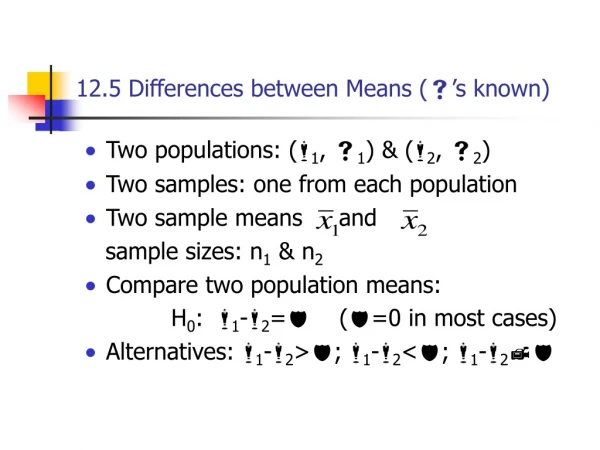
12.5 Differences between Means ( s ’s known). Two populations: ( 1 , 1 ) & ( 2 , 2 ) Two samples: one from each population Two sample means and sample sizes: n 1 & n 2 Compare two population means: H 0 : 1 - 2 = ( =0 in most cases)

12.5 Differences between Means ( s ’s known)
E N D
Presentation Transcript
12.5 Differences between Means (s’s known) • Two populations: (1, 1) & (2, 2) • Two samples: one from each population • Two sample means and sample sizes: n1 & n2 • Compare two population means: H0: 1-2= (=0 in most cases) • Alternatives: 1-2>; 1-2<; 1-2
Let’s go through a two sided alternative • H0: 1-2=0 vs HA: 1-2≠0 • Reject H0 if is too far from zero in either direction. • How far from zero might be if 1-2=0? • Sampling distribution of is asymptotically normal with mean 0 and standard deviation • We need to know
Fact: • If the sample means are from independent samples, then
Thus under certain assumptions: Correspondingly, a confidence interval for m1-m2 is
Assumptions • 1 & 2 are known • Normal populations or large sample sizes • Under null hypothesis is (asymptotically) standard normal
Example 12.4 • Two labs measure the specific gravity of metal. On average do the two labs give the same answer? 1 -- Population mean by lab1 2 -- Population mean by lab2 • H0: 1=2 vs HA: 12 • 1=0.02, n1=20, • 2=0.03, n2=25,
95% Confidence Interval from –0.014 to 0.016
Two-tailed Hypotheses Test • Two sample test • Rejection region: |Z|>z0.025=1.96 • Conclusion: Don’t reject H0.
Exercise • An investigation of two kinds of photocopying equipment showed that a random sample of 60 failures of one kind of equipment took on the average 84.2 minutes to repair, while a random sample of 60 failures of another kind of equipment took on the average 91.6 minutes to repair. If, on the basis of collateral information, it can be assumed that s1=s2=19.0 minutes for such data, test at the 0.02 level of significance whether the difference between these two sample means is significant.
12.6 Differences Between Means (unknown equal variances) • Large samples n130; n230 • Small samples 1. 1=2 2. 12
Large Samples • n130; n230 • Estimate 1 and 2 by s1 and s2 • Set
Small Samples • 1=2= unknown • Two populations are normal • Standard error • Estimate the common variance
Pooled standard deviation • Using both s12 and s22 toestimate 2, we combine these estimates, weighting each by its d.f.. The combined estimate of 2 is sp2, the pooled estimate: • Estimate by sp
Two-Sample T-test • T-test (t distribution with df=n1+n2-2) • 100(1-)% CI Hypothesized m1-m2
Example 12.5 • Compare blood pressures • Two populations: common variance • =0.05 • n1=10, s1=16.2, • n2=12, s2=14.3,
CI & test • sp=15.2 df=10+12-2=20 • Critical value t0.025=2.086 • t statistic: reject H0 if |t|>2.086 • Conclusion? Don’t Reject. • CI: -122.086(6.51)=-12 13.6 -1.6 to 25.6
What happens when variances are not equal? • Testing: H0: m1-m2=δ. • Normal population • s1 and s2 are not necessarily equal • s1 and s2 unknown
Two sample t-test with unequal variances d.f. =min(n1-1, n2-1)
Exercise • In a department store’s study designed to test whether or not the mean balance outstanding on 30-day charge accounts is the same in its two suburban branch stores, random samples yielded the following results: Use the 0.05 level of significance to test the null hypothesis m1-m2=0.
12.7 Paired Data 1982 study of trace metals in South Indian River. 6 random locations 5 3 1 6 2 4 T=top water zinc concentration (mg/L) B=bottom water zinc (mg/L) 1 2 3 4 5 6 Top 0.415 0.238 0.390 0.410 0.605 0.609 Bottom 0.430 0.266 0.567 0.531 0.707 0.716
One of the first things to do when analyzing data is to PLOT the data • This is not a useful way to plot the data. There is not a clear distinction between bottom water and top water zinc—even though Bottom>Top at all 6 locations. Top Bottom
A better way Top Bottom Connect points in the same pair.
A better way Bottom=Top The plot suggests that mBottom>mTop. Is it true?
That is equivalent to ask: is it true that mdifference>0? 1 2 3 4 5 6 Top 0.415 0.238 0.390 0.410 0.605 0.609 Bottom 0.430 0.266 0.567 0.531 0.707 0.716 D=B-T 0.015 0.028 0.177 0.121 0.102 0.107 Ho: mD=0 vs HA: mD>0
Doing a one-sided test Ho: mD=0 vs HA: mD>0 t0.05 at 5 d.f. is 2.015. So anything greater than 2.015 will be an evidence against H0. We reject H0: mB-T=0 in favor of HA: mB-T>0.
Another example • The average weekly losses of man-hours due to accidents in 10 industrial plants before and after installation of an elaborate safety program: • Plants 1 2 3 4 5 6 7 8 9 10 • Before 45 73 46 124 33 57 83 34 26 17 • After 36 60 44 119 35 51 77 29 24 11 diff(B-A) 9 13 2 5 -2 6 6 5 2 6 • Is the safety program effective? (level=0.05)
Two Populations: Before and After • Normal? • Independent? No, No
Normal Probability Plots • Small sizes • Skew to right somehow
Normal Probability Plot for Difference Looks better
Consider the Differences • Paired Observations:before and after the installation of safety program are from the same plants (dependent) • Data from different plants may be independent • Diff: 9 13 2 5 -2 6 6 5 2 6
Set up a Test—Paired T-Test • ‘effective’ means the program reduces the accidents, i.e., before > after (D>0) • =difference of average accidents H0: D=0 vs HA: D>0 The procedure is the same as the one- sample t-test Df=n-1
Paired t-test • One-tailed test • Critical value: df=9, t0.05=1.833 • Sample mean & standard deviation: • t-statistic: • Conclusion: reject H0 since t=4.03>1.833
