Is there any air down there? Using multiple 3D numerical models to

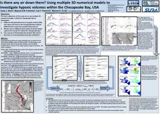
1. Is there any air down there? Using multiple 3D numerical models to investigate hypoxic volumes within the Chesapeake Bay, USA 1. Now at Delta Modeling Associates, Inc. San Francisco, CA. 2. Virginia Institute of Marine Science Gloucester Point, VA. 3. Old Dominium University Norfolk, VA Aaron J. Bever1, Marjorie A.M. Friedrichs2, Carl T. Friedrichs2, Malcolm E. Scully3: aaron@deltamodeling.com, margy@vims.edu, cfried@vims.edu Objectives: The main objectives of this work are to use multiple 3D numerical models within the Chesapeake Bay to investigate: What are the potential errors in hypoxic volume (HV) over space and time in the Chesapeake Bay Program (CBP) HV time-series from profile observations? Would more or different observation locations better capture the real 3D HV within the Chesapeake Bay? Can a group of Chesapeake Bay models help inform decisions on instrumentation and data collection? Methods: Three-dimensional dissolved oxygen (DO) fields were provided from the CH3D-ICM and ROMS models for 2004 and 2005. The ICM model is a full ecological model with at least 24 state variables, while the ROMS implementations used one of two single-equation oxygen formulations. We used, in summary: CH3D + ICM = CH3D hydrodynamic model + full ecological model (CE-QUAL-ICM) (ICM model grid, Z grid) ChesROMS + 1-Term = ROMS hydrodynamic model + Constant Respiration rate (ChesROMS model grid, low resolution, sigma grid) ChesROMS + Depth Dep. = ROMS hydrodynamic model + Depth Dependant Respiration rate (ChesROMS model grid, low resolution, sigma grid) CBOFS2 + 1-Term = ROMS hydrodynamic model + Constant Respiration rate (CBOFS2 model grid, high resolution, sigma grid) Different methods of calculating hypoxic volume from model DO simulations were used. 1) The total hypoxic volume from the 3D DO fields was calculated. 2) The CBP interpolator was used to calculate HV from discrete station location sets. These were the A) Absolute Match: Model estimates at the exact time and location as the available observations (~30-60 stations). B) Spatial Match: Model estimates as a synoptic snapshot using only these observed stations. C) All Stations: Model estimates using all possible CBP stations (~100, Fig. 1). And D) Station subsets chosen based on model results. HVs were also calculated using CBP station observations alone. Errors from only sampling discrete points Potential errors due to time-lags in sampling Stations based on model estimates of bottom DO. Fig. 2. Left Panels: The total modeled HV based on the 3D fields (blue), the absolute match (black), the spatial match (red), and the all stations (green). Horizontal lines (black) show the date range that the observed profiles were collected over. Vertical lines (red) show the range of stations spatial HV over the date range that the observed profiles were collected. The black dots are directly comparable to the observations. Right: Panels: Potential errors in the calculation of HV from discrete stations. Estimates of HV using discrete sets of stations underestimates the true 3D HV. There is little difference between the HV from the spatial match set and the set using all station locations. Because the profiles within each sampling cruise are collected over a period up to 2 weeks, the DO fields evolve during the sampling, creating a range of real synoptic HV snapshots over the time-period of each cruise (red lines). This potential temporal error is at least as important as the error from only sampling discrete stations. Fig. 5. Left Panels: The fraction of 2004 the models estimated bottom water to have a DO concentration of 2 mg/L or less. Right Panels: The standard deviation of the bottom dissolved oxygen concentrations, as a metric of the variability. These target diagrams show: Y axis= The bias of the stations HV in relation to the total modeled 3D HV. X axis= The unbiased RMS difference between the stations HV and the total modeled 3D HV. The closer to the center, the better a stations HV reproduced the total 3D hypoxic volume. Model results give information on potential instrument locations. For example, if using high time-resolution instruments, data can be collected where DO is low and the variability is high (circles), to get the most information out of the observations. Examples include the flanks of the channel in the middle reaches of the bay, and the lower Potomac River. Scale Stations HV by log10 function. Coefficients: a = 0.88, b = -1.1 CBOFS2 2005 is in progress. Fraction of station HV it missed 3D HV by. Negative = underestimate Total RMSD, 2004 or 2005 Because locations of hypoxia are controlled by bathymetry, a few strategic stations can represent the total 3D HV nearly as well as using 50 stations, or 32 in assumed optimal locations. These 13 stations can be profiled in 2-3 days, limiting the possible temporal errors in the HV calculations. A scaling factor can then be used with the set of 13 CBP stations predominantly in the main stem, further improving these HV estimates (green markers). Minimum 10 Stations Optimal 2 km3 cutoff Tributaries Fig. 1. Bathymetry and spatial extent of Chesapeake Bay and the tributaries. Circles are the CBP profile locations, those with red rings are the 13 stations that were used for HV estimates in Figs. 3, 4. The aspect ratio of the bay is stretched in the east-west direction, to better show the bathymetry and station locations. Fig.4. Figures showing how well the CBP13 stations set HV reproduced the 3D HV; showing the fraction of the CBP13 HV (Y axis) that these estimates, generally, underestimated the 3D HV. The left figure shows the original CBP13 HVs calculated from the model results, and the right figure shows the same comparison after the CBP13 HVs were all scaled by the exact same function. The equation of a best fit line is shown, along with the RMSD. The below equation shows the scaling function. Flanks Scaled HV = CBP13 + F(CBP13) *CBP13 Better Represent “Real” 3D HV Stations HV Fig. 3. Target diagram showing how well the total 3D HV from each model is reproduced by different stations sets. Sets correspond to; min10: 10 stations in the main stem, Flanks: The min10 stations plus the stations on the flanks, Trib.: The min10 stations plus those in the tributaries, Fl+Tr: The min10 plus the flanks and tributary stations, O1: Presumed optimal station locations for capturing hypoxia, CBP13: A set of 13 CBP stations, CBP13SC: The set of 13 CBP stations scaled to better match the total 3D hypoxic volume. Note: The scaling function was limited to only reduce the stations HV by a maximum of 1/4, to not reduce large HVs too far. i.e. F = max(F,-0.25) A scaling function was developed from a subset of CBP stations that created a better match with the real HV within the bay and reduced temporal and spatial uncertainties. The coefficients used here were insensitive to the specific subset of stations, showing the scaling function is relatively robust. Conclusions: The potential HV errors from time lags in data collection are similar to those from sampling discrete points, and the difference in HV estimates from assuming a synoptic snapshot or incorporating the absolute date and time the samples were collected (absolute compared to spatial) is larger than the differences from adding more stations (all compared to spatial). This implies sampling frequency may be more important than number of stations. Neither more nor better station locations are necessary to reasonably capture the true 3D HV. The models showed that the HV from a subset of 13 stations can be scaled to further improve the representation of the true 3D HV. The models can be used to determine locations for instrument/station placement that are tailored to the specific instrumentation and/or scientific questions. We would like to thank the many people who have provided us with model output and information on model implementations, model physics, etc, even if the models are not represented on this specific poster. Funding was provided by NOAA/IOOS via the SURA Super-Regional Testbed Project. Additional members of the Testbed’s Estuarine Hypoxia Team include C. Cerco (USACE), D. Green (NOAA-NWS), R. Hood (UMCES), L. Lanerolle (NOAA-CSDL), J. Levin (Rutgers), M. Li (UMCES), L. Linker (EPA), W. Long (UMCES), M. Scully (ODU), K. Sellner (CRC), J. Shen (VIMS), J. Wilkin, (Rutgers), and D. Wilson (NOAA-NCBO),