Download
1 / 50
500 likes | 701 Views
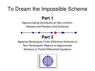
To Dream the Impossible Scheme. Part 1 Approximating Derivatives on Non-Uniform, Skewed and Random Grid Schemes Part 2 Applying Rectangular Finite Difference Schemes to Non-Rectangular Regions to Approximate Solutions to Partial Differential Equations.

E N D
To Dream the Impossible Scheme Part 1 Approximating Derivatives on Non-Uniform, Skewed and Random Grid Schemes Part 2 Applying Rectangular Finite Difference Schemes to Non-Rectangular Regions to Approximate Solutions to Partial Differential Equations
Approximating Derivatives on Non-Uniform, Skewed and Random, Grid Schemes Skewed Non-Uniform Random
Approximating Derivativesfrom a Data Table How do we approximate f’(.5)
Approximating Derivativesfrom a Data Table 2-Point Forward Difference Approximation
Approximating Derivativesfrom a Data Table 2-Point Backward Difference Approximation
Approximating Derivativesfrom a Data Table 2-Point Central Difference Approximation
Approximating Derivativesfrom a Data Table In Summary … so Far Which is right? Which is better?
Approximating Derivativesfrom a Data Table 3-PT FD Approx
Approximating Derivativesfrom a Data Table 4-PT CD Approximation Note the new compact notation:
Approximating Derivativesfrom a Data Table 5-PT FD Approximation:
Approximating Derivativesfrom a Data Table In Summary Which is the best approximation?
2-point FD: 2-point CD: 3-point FD: 4-point CD: 5-point FD: Estimates of the 1st Derivative (CRC)
2nd D,2-point CD : 3rd D, 4-point FD: 3rd D, 4-point CD: 4th D, 5-point FD: 4th D, 5-point CD: Estimates of Higher Order Derivatives (CRC)
Where do these Equations Come From • Derivation starts with the Taylor Series centered on x: • i.e: • Or in a shorthand form the you will see on the following slides:
Derivation of 2-Point BD Equation for the 1st Derivative on a Uniform Grid Start with Three 3-Term Taylor Series Expansions. Where: fn=f(x0+nδ) where δis the grid spacing. Note: Equation for f0is expanded for use in further derivation Note: Define 00=1
Derivation of 3-Point BD Equation for the 1st Derivative on a Uniform Grid Multiply Each Equation by a Weight ωn . Note: Error term dropped for the time being for brevity
Derivation of 3-Point BD Equation for the 1st Derivative on a Uniform Grid Sum up the Coefficients to Generate the 1st Derivative Expression .
Derivation of 3-Point BD Equation for the 1st Derivative on a Uniform Grid A little algebraic manipulation …
Derivation of 2-Point BD Equation for the 1st Derivative on a Uniform Grid And rewritten as a matrix equation … Note: A Vandermonde Matrix
Derivation of 3-Point BD Equation for the 1st Derivative on a Uniform Grid A General Vandermonde Matrix
Cofactor Expansion Determinant of a Vandermonde matrix Solving for ω-2 Using Cramer’s Rule
Derivation of 3-Point BD Equation for the 1st Derivative on a Uniform Grid Solve for the Remaining Weights. Now use weights to calculate the coefficient of the remainder term …
Derivation of 3-Point BD Equation for the 1st Derivative on a Uniform Grid Voila! .
Derivation of 3-Point BD Equation for the 2nd Derivative on a Uniform Grid Alter RHS Slightly….
Derivation of 5-PointCD Equation for the 3rd Derivative on a Uniform GriD (or, if I desire, anything up to the 4th Derivative) (or, if I desire, anything up to the 4th Derivative)
System will also Work for Skew Grid Schemes (i.e. use backward 1st and 4th point and forward 1st , 2nd, and 6th point to findthe 3rd derivative on a uniform grid) Note: The grid is “uniform”, the spacing between the points is not.
A General Matrix System (for an r-point approximation for the ith derivative) an: integer that describes position of grid point with respect to center point (i.e. anΔx).
Which “Simplifies” to: Cofactor Expansion About the 1st Column and The (i+1)th Row Determinant of a Vandermonde matrix
Vandermonde Matrix with the rth row and nth column removed. Minor of the Vandermonde Matrix With the (i+1)th row and nth column removed (from previous slide). Schur polynomial of order r-i-1 Turning our Attention to the Numerator … T. Ernst, Generalized Vendermonde Systems of Equations. Mathematics of Computation, 24, (1970) 893-903. I.G. Macdonald, Symmetric Functions and Hall Polynomials, Oxford Mathematical Mongraphs, Second Ed. 1995. S.D. Marchi, Polynomials arising in factoring generalized Vandermonde determinants: An algorthm for computing their coefficients, The Mathematical and Computer Modeling, 34 (2003) 280-287.
Schur Polynomial det(V) Therefore …
Finally … Where ωn is the nth weight for an r-point estimate of the ith derivative with grid points whose relative position to the center is given by {a1, …, ar} and grid spacing is δ.
Recall the Earlier Example … (i.e. use backward 1st and 4th point and forward 1st , 2nd, and 6th point to estimatethe 3rd derivative on a uniform grid) Note: The grid is “uniform”, the spacing between the points is not.
The Extension to Random Grids… A slight adjustment to this equation will accomplish this. Let δ=1 and ai be the position from the point of interest.
Applying Finite Difference Schemes to Non-Rectangular Regions
The Wave Equationon a Circular Membrane Object: Solve analytically using the polar from of the wave equation. Then compare to a numerical finite difference approximation that superimposes a rectangular grid on the circle. Note that the grid size varies from point to point on the circle.
Wave Equation: Rectangular Form: Polar Form: Polar Form: (Radial Symmetry) The Wave Equation
PDE (ω=1, 0≤r ≤1): Boundary Conditions: Initial Conditions: Boundary/Initial Conditions
Analytic Solution Jm: Bessel Function of the First Kind of order m μmn: Is the ntheigenvalue of Jm
Numeric Solution Since the grid is rectangular, use the rectangular form of the wave equation: The discrete form of this equation from finite difference methods Note: Based on 3-point central difference formulations of the spatial terms. Note: Based on 3-point backward difference formulation in time. Note: The time grid is uniform.
Numeric Solution Time Stepping: Stability Requirement: Δt ≤ smallest grid increment