Download
1 / 34
340 likes | 483 Views
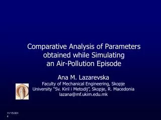
Comparative Analysis of Parameters obtained while Simulating an Air-Pollution Episode. Ana M. Lazarevska Faculty of Mechanical Engineering, Skopje University “Sv. Kiril i Metodij”, Skopje, R. Macedonia lazana@mf.ukim.edu.mk. Engaged set of software tools:.

E N D
Comparative Analysis of Parameters obtained while Simulating an Air-Pollution Episode Ana M. LazarevskaFaculty of Mechanical Engineering, Skopje University “Sv. Kiril i Metodij”, Skopje, R. Macedonialazana@mf.ukim.edu.mk
Engaged set of software tools: preprocessors, models, postprocessors, graphical visualization Overview Application areas of Air Quality, Pollutant Dispersion and Transport Models Problem Description Necessary input data for simulating the air pollution episode (APE) Results Conclusion Comparative Analysis of Parameters obtained while Simulating an APE
2. Policy support - - air quality assessment studies- forecasting the effect of abatement measures - combined use of AQM with other environmental models 3. Public information - - on-line information - possible occurrence of smog episodes - on-line forecasting - reciprocal exchange of smog information between countries 4. Scientific research - - description of dynamic effects - simulation of complex chemical processes involving air pollutants. - for practical applications - high requirement o computational effort diagnosis, analysis and prognosis Application areas ofAir Quality, Pollutant Dispersion and Transport Models 1. Regulatory purposes - issuing emission permits Comparative Analysis of Parameters obtained while Simulating an APE
Problem Description Simulation of an SO2 air pollution episode • Analyzed Region – Grid, Mesh • Selection of an episode for simulation • Selection of a simulation tool –CALPUFF vs. FLUENT • Numerical simulation of the selected air pollution episode over the region of interest (FLUENT, CALPUFF) • Comparative analysis of the parameters engaged Comparative Analysis of Parameters obtained while Simulating an APE
geo-physical parameters • emission parameters • meteorological parameters • receptor data Simulation of an SO2 air pollution episodeAnalyzed region and episode - selectioncriteria • Skopje is the capitol of the R. Macedonia, (30% of the population, main industrial center)- concentration of polluters - represent of APEs • Simultaneous existence of min.necessary input data Comparative Analysis of Parameters obtained while Simulating an APE
Comparative Analysis of Parameters obtained while Simulating an APE
Simulation of an SO2 air pollution episodeSelection of a simulation tool CALPUFF approach – multi layer, multi species, non-steady-state puff dispersion model - simulates effects of varying (xi,t) meteorological conditions on pollutant transport, transformation and removal – contains algorithms/modules for near-source effects (building downwash, transitional plume rise, sub-grid scale terrain interactions), longer range effects (pollutant removal, chemical transformation, over-water transport etc.) Comparative Analysis of Parameters obtained while Simulating an APE
C(s)ground level concentration [g/m3]. Q(s)pollutant mass in the puff [g]. sx,y,z(s)standard deviation of the Gaussian distribution (along/across wind and vertical direction) [m] da,c(s)distance from puff center to the receptor (along / across wind direction) [m] g(s)vertical term (multiple reflection from top of ML and surface) Hepuff center's effective height above ground [m]. hML height [m]. Comparative Analysis of Parameters obtained while Simulating an APE
Simulation of an SO2 air pollution episodeSelection of a simulation tool (cont.) FLUENT provides comprehensive modeling capabilities for – incompressible and compressible fluid flow problems, –laminar and turbulent fluid flow problems. –Steady-state or transient analyses –models for transport phenomena (heat transfer and chemical reactions) –combined with ability to model complex geometries. in order to allow comparison – “try-to-imitate” CALMET/CALPUFF approach Comparative Analysis of Parameters obtained while Simulating an APE
Simulation of an SO2 air pollution episodeSelection of a simulation tool(cont.) – grid – horizontally / vertically – same distancing – fields of meteorological parameters modeled, as much as the solver allows, similarly to the approach in CALMET (“hour–by–hour”) – boundary conditions – main flow: vel. & press. inlet – modeling of pollution transport (here w.o. chem.reac.) – species transport with Discrete Phase Model (DPM), which performs Lagrangian trajectory calculations for dispersed phases (particles, droplets, or bubbles). 1 step: solution of the main flow 2 step: emissions modeled as point injections 3 step: coupling with the continuous phase (possible) Comparative Analysis of Parameters obtained while Simulating an APE
Mass Conservation Equation Sm mass added to the continuous phase from the dispersed second phase and any user-defined sources. Transport Equations for the Standard k-e Model Gk generation of turbulence kinetic energy due to mean velocity gradientsGb generation of turbulence kinetic energy due to buoyancy YM contribution of fluctuating dilatation in compressible turbulence to overall dissipation rate,C1e, C2e, C3e constants. sk, se turbulent Prandtl numbers for k and e, respectively. Sk, Seuser-defined source terms. Comparative Analysis of Parameters obtained while Simulating an APE
Species Transport Equations Yilocal mass fraction of each species, Rinet rate of production by chemical reaction Sirate of creation by addition from the dispersed phase plus any user-defined sources. Heat Transfer to the Droplet Cpdroplet heat capacity (J/kg-K) Tpdroplet temperature (K) hconvective heat transfer coefficient (W/m2 K)Ttemperature of continuous phase (K)dmp/dtrate of evaporation (kg/s)hfglatent heat (J/kg)epparticle emissivity (dimensionless)sStefan-Boltzmann constant (5.67 10-8 W/m2 K4) qRradiation temperature, Comparative Analysis of Parameters obtained while Simulating an APE
Meteorological and Geophysical PreprocessorsExcel & VBasic CALMET Meteorological model CALPUFF Dispersion model CALPOST Postprocessor PRTMET Meteorological postprocessor MATLAB Statistics, AnalyzeGraphical visualization, Animation Geophysical PreprocessorGAMBIT Meteorological boundary conditions (main flow) FLUENT Solution of the main flow FLUENT Solution of the discrete phase FLUENT AnalyzeGraphical visualization, Animation, Statistics Comparative Analysis of Parameters obtained while Simulating an APE
FLUENT and CALPUFF Mesh of the Region Comparative Analysis of Parameters obtained while Simulating an APE
Simulation of an SO2 air pollution episodeNecessary input data for simulating the APE 1. Geophysical - surface elevation, LUC, surface roughness 2. Meteorological - surface and upper air soundings - modeled surface and upper air data 3. Emission data - flow and geometry properties modeled emission data 4. Receptor data - ground concentrations 5. Mixture properties - species (FLUENT) Comparative Analysis of Parameters obtained while Simulating an APE
z [m] Comparative Analysis of Parameters obtained while Simulating an APE
z [m] Comparative Analysis of Parameters obtained while Simulating an APE
1. 3D hourlyfields of meteorological data p, r, T, |u|, u(direction), r[%] Postprocessing 2. ground concentrations of modeled species 3. Development of the APE Comparative Analysis of Parameters obtained while Simulating an APE
Comparative Analysis of Parameters obtained while Simulating an APE
Comparative Analysis of Parameters obtained while Simulating an APE
Comparative Analysis of Parameters obtained while Simulating an APE
Comparative Analysis of Parameters obtained while Simulating an APE
Comparative Analysis of Parameters obtained while Simulating an APE
Comparative Analysis of Parameters obtained while Simulating an APE
Comparative Analysis of Parameters obtained while Simulating an APE
Comparative Analysis of Parameters obtained while Simulating an APE
Jul 12, 2004 Comparative Analysis of Parameters obtained while Simulating an APE
Jul 12, 2004 Comparative Analysis of Parameters obtained while Simulating an APE
Jul 12, 2004 Comparative Analysis of Parameters obtained while Simulating an APE
Jul 12, 2004 Comparative Analysis of Parameters obtained while Simulating an APE
Comparative Analysis of Parameters obtained while Simulating an APE
Results 1. Formation and Development Trends of the APE are maintained 2. Performance Comparison: FLUENT vs. CALPUFF • Advantages: a. aside of the geometry/mesh preprocessor GAMBIT, FLUENT alone conducts the complete calculation of flow and species parameters • b. Particle tracking avlb. within FLUENT • c. 3D field of species fraction - Disadvantages: selecting/tuning the proper model in FLUENT might turn out to be a time consuming and difficult task Comparative Analysis of Parameters obtained while Simulating an APE
Conclusion • The comparative analysis implies a possibility of supplementing the both software packages, aiming a better quality of the output • However, due to the poor quality of input parameters, the analysis shows that formation and development of an APE can be predicted only qualitatively, i.e. onlynotificationofexistence / prediction of an APE • The outcome certainty is a function of the input parameters quality Comparative Analysis of Parameters obtained while Simulating an APE