Download
1 / 53
590 likes | 887 Views
Prediction of protein contact maps. Piero Fariselli. Department of Biology University of Bologna. From Sequence to Function. >BGAL_SULSO BETA-GALACTOSIDASE Sulfolobus solfataricus. MYSFPNSFRFGWSQAGFQSEMGTPGSEDPNTDWYKWVHDPENMAAGLVSG DLPENGPGYWGNYKTFHDNAQKMGLKIARLNVEWSRIFPNPLPRPQNFDE

E N D
Prediction of protein contact maps Piero Fariselli Department of Biology University of Bologna
From Sequence to Function >BGAL_SULSO BETA-GALACTOSIDASE Sulfolobus solfataricus. MYSFPNSFRFGWSQAGFQSEMGTPGSEDPNTDWYKWVHDPENMAAGLVSG DLPENGPGYWGNYKTFHDNAQKMGLKIARLNVEWSRIFPNPLPRPQNFDE SKQDVTEVEINENELKRLDEYANKDALNHYREIFKDLKSRGLYFILNMYH WPLPLWLHDPIRVRRGDFTGPSGWLSTRTVYEFARFSAYIAWKFDDLVDE YSTMNEPNVVGGLGYVGVKSGFPPGYLSFELSRRHMYNIIQAHARAYDGI KSVSKKPVGIIYANSSFQPLTDKDMEAVEMAENDNRWWFFDAIIRGEITR GNEKIVRDDLKGRLDWIGVNYYTRTVVKRTEKGYVSLGGYGHGCERNSVS LAGLPTSDFGWEFFPEGLYDVLTKYWNRYHLYMYVTENGIADDADYQRPY YLVSHVYQVHRAINSGADVRGYLHWSLADNYEWASGFSMRFGLLKVDYNT KRLYWRPSALVYREIATNGAITDEIEHLNSVPPVKPLRH Genomic sequences Protein structures Protein sequences Functional Genomics and Proteomics Protein functions
The Protein Folding T T C C P S I V A R S N F N V C R L P G T P E A L C A T Y T G C I I I P G A T C P G D Y A N
The Data Bases of Sequences and Structures EMBL: 195,241,608 sequences 292,078,866,691nucleotides >BGAL_SULSO BETA-GALACTOSIDASE Sulfolobus solfataricus. MYSFPNSFRFGWSQAGFQSEMGTPGSEDPNTDWYKWVHDPENMAAGLVSG DLPENGPGYWGNYKTFHDNAQKMGLKIARLNVEWSRIFPNPLPRPQNFDE SKQDVTEVEINENELKRLDEYANKDALNHYREIFKDLKSRGLYFILNMYH WPLPLWLHDPIRVRRGDFTGPSGWLSTRTVYEFARFSAYIAWKFDDLVDE YSTMNEPNVVGGLGYVGVKSGFPPGYLSFELSRRHMYNIIQAHARAYDGI KSVSKKPVGIIYANSSFQPLTDKDMEAVEMAENDNRWWFFDAIIRGEITR GNEKIVRDDLKGRLDWIGVNYYTRTVVKRTEKGYVSLGGYGHGCERNSVS LAGLPTSDFGWEFFPEGLYDVLTKYWNRYHLYMYVTENGIADDADYQRPY YLVSHVYQVHRAINSGADVRGYLHWSLADNYEWASGFSMRFGLLKVDYNT KRLYWRPSALVYREIATNGAITDEIEHLNSVPPVKPLRH UNIPROT: 428 650sequences 154'416'236 residues PDB: 68000 structures membrane proteins 1% November/2009
What is a multiple alignment ? The short answer is this - VTISCTGSSSNIGAG-NHVKWYQQLPG VTISCTGTSSNIGS--ITVNWYQQLPG LRLSCSSSGFIFSS--YAMYWVRQAPG LSLTCTVSGTSFDD--YYSTWVRQPPG PEVTCVVVDVSHEDPQVKFNWYVDG-- ATLVCLISDFYPGA--VTVAWKADS-- AALGCLVKDYFPEP--VTVSWNSG--- VSLTCLVKGFYPSD--IAVEWESNG--
Evolutionary information • Multiple Sequence Alignment (MSA) of similar sequences • Sequence profile: for each position a 20-valued vector contains the aminoacidic composition of the aligned sequences. 1 Y K D Y H S - D K K K G E L - - 2 Y R D Y Q T - D Q K K G D L - - 3 Y R D Y Q S - D H K K G E L - - 4 Y R D Y V S - D H K K G E L - - 5 Y R D Y Q F - D Q K K G S L - - 6 Y K D Y N T - H Q K K N E S - - 7 Y R D Y Q T - D H K K A D L - - 8 G Y G F G - - L I K N T E T T K 9 T K G Y G F G L I K N T E T T K 10 T K G Y G F G L I K N T E T T K A 0 0 0 0 0 0 0 0 0 0 0 10 0 0 0 0 C 0 0 0 0 0 0 0 0 0 0 0 0 0 0 0 0 D 0 0 70 0 0 0 0 60 0 0 0 0 20 0 0 0 E 0 0 0 0 0 0 0 0 0 0 0 0 70 0 0 0 F 0 0 0 10 0 33 0 0 0 0 0 0 0 0 0 0 G 10 0 30 0 30 0 100 0 0 0 0 50 0 0 0 0 H 0 0 0 0 10 0 0 10 30 0 0 0 0 0 0 0 K 0 40 0 0 0 0 0 0 10 100 70 0 0 0 0 100 I 0 0 0 0 0 0 0 0 30 0 0 0 0 0 0 0 L 0 0 0 0 0 0 0 30 0 0 0 0 0 0 0 0 M 0 0 0 0 0 0 0 0 0 0 0 0 0 60 0 0 N 0 0 0 0 10 0 0 0 0 0 30 10 0 0 0 0 P 0 0 0 0 0 0 0 0 0 0 0 0 0 0 0 0 Q 0 0 0 0 40 0 0 0 30 0 0 0 0 0 0 0 R 0 50 0 0 0 0 0 0 0 0 0 0 0 0 0 0 S 0 0 0 0 0 33 0 0 0 0 0 0 10 10 0 0 T 20 0 0 0 0 33 0 0 0 0 0 30 0 30 100 0 V 0 0 0 0 10 0 0 0 0 0 0 0 0 0 0 0 W 0 10 0 0 0 0 0 0 0 0 0 0 0 0 0 0 Y 70 0 0 90 0 0 0 0 0 0 0 0 0 0 0 0 MSA sequence position Sequence profile
3D structure prediction of proteins New folds Existing folds Building by homology Ab initio prediction Threading 0 10 20 30 40 50 60 70 80 90 100 Homology (%)
Contacts and Contact Maps F 156 V 299 I 269 F 297 V 271 I 240 V 238 Contact definition
1. Based on Ca 2. Based on Cb 3. All-atom (without Hydrogens) Protein contact definitions:
From the 3D structure to the contact map Given a protein of length L, and a square matrix M of dimension L L For each pair of residue i and j calculate distance between i and j if distance < threshold put 1 in the cell M(i,j) otherwise put 0 in the cell M(i,j)
Computation of Contact Maps From 3D Structure TTCCPSIVARSNFNVCRLPGTPEAICATYTGCIIIPGATCPGDYAN TTCCPSIVARSNFNVCRLPGTPEAICATYTGCIIIPGATCPGDYAN F 156 To Contact Map V 299 I 269 F 297 V 271 I 240 V 238
Protein Structural Classes All-b All-a a /b a + b
2 4 1 3 3 4 2 1 An Example of a Contact map (All-a)
C N An Example of Contact map (a + b)
From the contact map to the 3D structure • Two methods have been proposed : • Bohr et al., “Protein Structure from distance Inequalities” J.Mol. Biol. 1993, 231:861-869 => based on a steepest descent procedure • Vendruscolo and Domany Fold. Des. 1998, 2:295-306=> based on a modified Metropolis procedure
6pti Reconstruction Efficiency (58 residues) Vendruscolo and Domany Fold. Des. 1998 RMSD M (Number of random flipping) At M= 200 No of eliminated true contacts 6 % real contacts No of added false contacts 52 % real contacts
From the contact map to the 3D structure: the reconstruction efficiency
3-D Modelling through Contact Maps example: Bacteriorhodopsin Model N 1QHJ (1.9 Å) Contact map C RMSD = 2.5 Å
MARC efficiency in 3D reconstruction from the protein contact map after progressive elimination of true contacts (6pti)
MARC efficiency in 3D reconstruction after progressive addition of wrong contacts to a protein contact map with 30 % of true contacts (6pti)
Prediction of Contact Maps Several methods have been applied: • Bohr et al., FEBS 1990 261:43-46=> based on neural networks • Göbel et al., PROTEINS 1994 18: 309-317=> based on correlated mutations in proteins • Thomas et al., Prot. Eng. 1996 9: 941-948=> based on a statistical method and evolution information • Olmea and Valencia Fold. Des. 1997 2:S25-S32 => based on correlated mutations and other information • Fariselli and Casadio Prot. Eng 1999 12:15-21=> based on neural networks and evolutionary information • Fariselli et al., CASP4/ and Prot. Eng. in press=> Neural networks and other information • Pollastri and Baldi al., Bioinformatics 2002 18 S62-S70=> Recurrent Neural networks
Relevant points • Contact Threshold • Sequence separation (or sequence gap) • No of contacts vs No of non-contacts
16 Å The Contact Threshold
16 Å 12 Å The Contact Threshold
16 Å 12 Å 8 Å The Contact Threshold
16 Å 12 Å 8 Å 6 Å The Contact Threshold
40 1 100 20 Sequence separation …VTISCTGSSSNIGAGNHVKWYQQLPG…
The Sequence Separation example of a sequence separation = 10 residues 2
Frequency distribution of the real and hypothetical contacts as a function of sequence separation
Relation between the number of contacts and the protein length Number of contacts Protein length
Evaluation of the efficiency of contact map predictions • 1) Accuracy: • A = Ncp* / Ncp • where Ncp* and Ncp are the number of correctly assigned contacts and that of total predicted contacts, respectively. • 2) Improvement over a random predictor : • R = A / (Nc/Np) • where Nc/Np is the accuracy of a random predictor ; Nc is the number of real contacts in the protein of length Lp, and Np are all the possible contacts • 3) Difference in the distribution of the inter-residue distances in the 3D structure for predicted pairs compared with all pair distances in the structure (Pazos et al., 1997): • Xd=i=1,n(Pic - Pia ) / n di • where n is the number of bins of the distance distribution (15 equally distributed bins from 4 to 60Å cluster all the possible distances of residue pairs observed in the protein structure); di is the upper limit (normalised to 60 Å) for each bin, e.g. 8 Å for the 4 to 8 Å bin; Pic and Pia are the percentage of predicted contact pairs (with distance between diand di-1 ) andthat of all possible pairs respectively
Tools out of machine learning approaches Neural Networks Training Prediction Data Base Subset New sequence TTCCPSIVARSNFNVCRLPGTPEAICATYTGCIIIPGATCPGDYAN General rules Known mapping Prediction
Contact definition used: • Cb - Cb distance < 0.8 nm • Sequence gap > 7 residues
The database of proteins used to train and test the contact map predictors.
Neural Network-based predictor • 1 output neuron (contact/non-contact) • 1 hidden layer with 8 neurons • Input layer with 1071 input neurons : • Ordered residue pairs (1050 neurons) • Secondary structures (18 neurons) • Correlated mutations (1 neuron) • Sequence conservation (2 neurons)
Representation of the input coding based on ordered couples. (A) An alignment of 5 (hypothetical) sequences they are represented in a HSSP file (Sander and Schneider, 1991). i and j stand for the positions of the two residues making or not making contact (A and D in the leading sequence or sequence 1). (B) Single sequence coding. The position representing the couple (AD) in the vector is set to 1.0 while the other positions are set to 0. (C) Multiple sequence coding. For each sequence in the alignment (1 to 5 in the scheme in A) a couple of residues in position i and j is counted. The final input coding representing the frequency of each couple in the alignment is normalized to the number of the sequences
1 MVKGPGLYTDIGKKARDLLYKDYHSDKKFTISTYSPTGVAITSS 2 MVKGPGLYSDIGKRARDLLYRDYQSDHKFTLTTYTANGVAITST 3 MVKGPGLYTEIGKKARDLLYRDYQGDQKFSVTTYSSTGVAITTT N sequences j i 1 MVKGPGLYTDIGKKARDLLYKDYHSDKKFTISTYSPTGVAITSS 2 MVKGPGLYSDIGKRARDLLYRDYQSDHKFTLTTYTANGVAITST 1 MVKGPGLYTDIGKKARDLLYKDYHSDKKFTISTYSPTGVAITSS 3 MVKGPGLYTEIGKKARDLLYRDYQGDQKFSVTTYSSTGVAITTT 2 MVKGPGLYSDIGKRARDLLYRDYQSDHKFTLTTYTANGVAITST 3 MVKGPGLYTEIGKKARDLLYRDYQGDQKFSVTTYSSTGVAITTT M = N·(N-1)/2 couples S : McLachlan substitution matrix S(T;S) S(T;T) S(S;T) S(I;L) S(I;V) S(L;V) Vj Vi M-valued vectors: Correlation: Correlated mutations Multiple sequence alignment
The neural network architecture for prediction of contact maps
Accuracy of contact map prediction using a cross-validated data set (170 proteins) No of proteins Accuracy