Download
1 / 28
280 likes | 400 Views
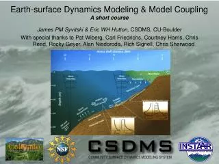
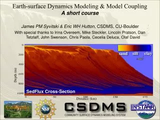
Earth-surface Dynamics Modeling & Model Coupling A short course. James PM Syvitski & Eric WH Hutton, CSDMS, CU-Boulder With special thanks to Jasim Imran, Gary Parker, Marcelo Garcia, Chris Reed, Yu’suke Kubo, Lincoln Pratson. after A. Kassem & J. Imran.

E N D
Earth-surface Dynamics Modeling & Model Coupling A short course James PM Syvitski & Eric WH Hutton, CSDMS, CU-Boulder With special thanks to Jasim Imran, Gary Parker, Marcelo Garcia, Chris Reed, Yu’suke Kubo, Lincoln Pratson after A. Kassem & J. Imran
Module 6: Density Currents, Sediment Failure & Gravity Flows ref: Syvitski, J.P.M. et al., 2007. Prediction of margin stratigraphy. In: C.A. Nittrouer, et al. (Eds.) Continental-Margin Sedimentation: From Sediment Transport to Sequence Stratigraphy. IAS Spec. Publ. No. 37: 459-530. Density Currents (2) Hyperpycnal Modeling (11) Sediment Failure Modeling (2) Gravity Flow Decider (1) Debris Flow Modeling (3) Turbidity Current Modeling (6) Summary (1) DNS simulation, E. Meiberg Earth-surface Dynamic Modeling & Model Coupling, 2009
Density-cascading occurs where shelf waters are made hyper-dense through: cooling (e.g. cold winds blowing off the land), or salinity enhancement (e.g. evaporation through winds, brine rejection under ice) Shelf Flows converge in canyons and accelerate down the slope. Currents are long lasting, erosive & carry sediment downslope as a tractive current, or as turbidity current. Earth-surface Dynamic Modeling & Model Coupling, 2009
POC: Dan Orange Cold water enters canyon across south rim. Erosive current generates furrows. Sand and mud carried by currents. Earth-surface Dynamic Modeling & Model Coupling, 2009
Dynamic model based on layer-averaged, 3-equations model of Parker et al. (1986) • Able to simulate time-dependent flows at river mouth • Data input: RM velocity, depth, width, sediment concentration. • Predicts grain size variation within a turbidite bed • Applicable to complex bathymetry with upslope SAKURA for modeling hyperpycnal flows after Y. Kubo Earth-surface Dynamic Modeling & Model Coupling, 2009
The model employs… 1. layer-averaged, 3-equations model with variation in channel width 2. Eulerian type (fixed) grid, with staggered cell C, H cell center U cell boundary Good for mass conservation 3. Two-step time increments Earth-surface Dynamic Modeling & Model Coupling, 2009
Mixing of freshwater and seawater Hyperpycnal flows in the marine environment involve freshwater and the sediment it carries mixing with salt water. River water enters the marine basin with a density of 1000 kg/m3, where it mixes with ocean water having a density typically of 1028 kg/m3. This mixing increases the fluid density of a hyperpycnal current, and alters the value of C and R, where where r is density of the fluid in the hyperpycnal current, rsw is density of the ambient seawater, rf is density of the hyperpycnal current (sediment and water), and rs is grain density Earth-surface Dynamic Modeling & Model Coupling, 2009
4. TVD scheme for spatial difference uses… • Uses 1st order difference scheme for numerically unstable area and higher order scheme for stable area • Avoids numerical oscillation with relatively less numerical diffusion • Possibly causes break of conservation law →used only in momentum equation. 5. Automatic estimation of dt dtis determined from adx/Umax at every time step with the value of safety factor agiven in an input file. 6. Variable flow conditions at river mouth • Input flow conditions are given at every SedFlux time step • When hyperpycnal condition lasts multiple time steps, a single hyperpycnal flow occurs with is generated from combined input data. Earth-surface Dynamic Modeling & Model Coupling, 2009
1. Removal rate, l Fdeposition = C Hl dt Equations for rate of deposition Steady rate of deposition regardless of flow conditions 2. Settling velocity, ws Fdeposition = Cb wsdt (Cb =2.0 C) Critical shear stress tc is not reliable Fdeposition = Cb wsdt (1-t/tc) 3. Flow capacity, Gz Fdeposition = wsdt ( C H - Gz) /H Earth-surface Dynamic Modeling & Model Coupling, 2009
Steady state profile of suspended sediment Amount of suspended sediments that a flow can sustain Flow capacity, Gz Critical flow velocity The excess amount of suspension start depositing when the total amount of suspended sediments exceeds the capacity. (Hiscott, 1994) Earth-surface Dynamic Modeling & Model Coupling, 2009
Experimental Results input 0.6, 0.9, 1.2 m from the source 0.3 m < thickness < 0.5 m 2.4, 3.0, 3.3, 3.6 m from the source thickness < 0.2 m Earth-surface Dynamic Modeling & Model Coupling, 2009
Continuous flow Jurassic Tank SedFlux Large pulse Small pulses Earth-surface Dynamic Modeling & Model Coupling, 2009
Multiple basins ---of the scale of Texas-Louisiana slope deeptow.tamu.edu/gomSlope/GOMslopeP.htm Earth-surface Dynamic Modeling & Model Coupling, 2009
A 2D SWE model application to the Eel River flood Imran & Syvitski, 2000, Oceanography 70 cm/s A 1D integral Eulerian model application to flows across the Eel margin sediment waves Lee, Syvitski, Parker, et al. 2002, Marine Geol. Earth-surface Dynamic Modeling & Model Coupling, 2009
FLUENT-modified FVM-CFD application Khan, Imran, Syvitski, 2005, Marine Geology Berndt et al. 2006 Earth-surface Dynamic Modeling & Model Coupling, 2009
F SEDIMENT FAILURE MODEL Examine possible elliptical failure planes Calculate sedimentation rate (m) at each cell Calculate excess pore pressure ui Gibsonui = g’zi A-1 where A = 6.4(1-T/16)17+1 T ≈ m2t/Cv and Cv = consolidation coefficient or use dynamic consolidation theory Earth-surface Dynamic Modeling & Model Coupling, 2009
SEDIMENT FAILURE MODEL 4) Determine earthquake load (horizontal and vertical acceleration) 5) Calculate JANBU Factor of Safety, F: ratio of resisting forces (cohesion and friction) to driving forces (sediment weight, earthquake acceleration, excess pore pressure) JANBU METHOD OF SLICES Where FT = factor of safety for entire sediment volume (with iterative convergence to a solution); bi=width of ith slice; ci=sediment cohesion; = friction angle; Wvi=vertical weight of column = M(g+ae); =slope of failure plane; Whi=horizontal pull on column = Mae; g=gravity due to gravity; ae=acceleration due to earthquake; M =mass of sediment column, ui= pore pressure. 6) Calculate the volume & properties of the failure: in SedFlux the width of the failure is scaled to be 0.25 times the length of the failure Determine properties of the failed material and decide whether material moves as a debris flow or turbidity current Earth-surface Dynamic Modeling & Model Coupling, 2009
Sediment Gravity Flow DeciderDebris Flow or Turbidity Current? • Properties of a failed mass determine the gravity flow dynamics. • If failed material is clayey (e.g. > 10% clay), then the failed mass is transported as a debris flow. Clay content is a proxy for ensuring low hydraulic conductivity and low permeability and thus the generation of a debris flow with viscoplastic (Bingham) rheology. • If the material is sandy, or silty with little clay (e.g.< 10% clay) then the failed sediment mass is transported down-slope as a turbidity current, where flow accelerations may cause seafloor erosion and this entrained sediment may increase the clay content of the flow compared to the initial failed sediment mass. Deposition of sand and silt along the flow path may result in the turbidity current transporting primarily clay in the distal reaches along the flow path. Earth-surface Dynamic Modeling & Model Coupling, 2009
Governing equations of the Lagrangian form of the depth-averaged debris flow equations: height of flow (1a) is inversely proportional to its velocity (1b). Continuity Momentum (shear (s) layer) Momentum (a) is balanced by weight of the flow scaled by seafloor slope (b); fluid pressure forces produced by variations in flow height (2c); and frictional forces (d). Momentum (plug flow (p) layer) h=height; U=layer-averaged velocity; g is gravity; S is slope; rw is density of ocean water; rm is density of mud flow; tm is yield strength, and mm is kinematic viscosity. Earth-surface Dynamic Modeling & Model Coupling, 2009
Given these governing equations for a debris flow, the dynamics do not allow the seafloor to be eroded. Thus the grain size of the final deposit is equal to the homogenized grain size of the initial failed sediment mass. Shear strength Runout Viscosity Runout Earth-surface Dynamic Modeling & Model Coupling, 2009
Failure Cohesion Shear strength Viscosity Friction angle load, ffriction angle, tshear strength, e void ratio, PI plasticity index, D grain size rr relative density Debris flow “Global” Sediment Properties • Coefficient of consolidation • Cohesion • Friction angle • Shear strength • Sediment viscosity “Local” Sediment Propertiesrelationships on a cell by cell basis Earth-surface Dynamic Modeling & Model Coupling, 2009
Four layer-averaged turbidity current conservation equations in Lagrangian form Fluid continuity (with entrainment) Sediment continuity Exner Equation Momentum = Gravity - Pressure - Friction Turbulent kinetic energy Dissipat. viscosity Resusp. Energy Entrainment Energy Bed Erosion Energy Energy Earth-surface Dynamic Modeling & Model Coupling, 2009
Chris Reed, URS Earth-surface Dynamic Modeling & Model Coupling, 2009
Pratson et al, 2001 C&G Earth-surface Dynamic Modeling & Model Coupling, 2009
3-Equation Model 4-Equation Model height velocity concentration Earth-surface Dynamic Modeling & Model Coupling, 2009
Turbidity current on a fjord bottom (Hay, 1987) Significant levee asymmetry High superelevation of flow thickness Application of Fluent 2D FVM –CFD model to modeling a turbidity current on a meandering bed (Kassem & Imran, 2004) Very mild lateral topography Earth-surface Dynamic Modeling & Model Coupling, 2009
Lateral flow field in a straight unconfined section. Density field at a bend in a unconfined section Flow field at a bend in a unconfined section Kassem & Imran, 2004 Very weak circulation cell Earth-surface Dynamic Modeling & Model Coupling, 2009
Density Currents, Sediment Failure & Gravity Flows Summary Density Currents: may interact with seafloor: RANS? Hyperpycnal Flow Models: 3eqn 1Dx & 2Dxy Lagrangian SWE; 3D FVM Sediment Failure Model: Janbu MofS FofS model + excess pore pressure model + material property model Gravity Flow Decider: material property model Debris Flow Model: Bingham, Herschel-Buckley, Bilinear rheologies; 1Dx 2-layer Lagrangian Turbidity Current Models: 3eqn & 4eqn 1Dx SWE; 3D FVM CFD (as a test try to translate this slide) Earth-surface Dynamic Modeling & Model Coupling, 2009