Download
1 / 51
510 likes | 608 Views
An Efficient Power-Aware Scheduling Algorithm for the Multiprocessor Platform. Lecture 6. This talk is based on the paper.

E N D
An Efficient Power-Aware Scheduling Algorithmfor the Multiprocessor Platform Lecture 6 Lecture 6
This talk is based on the paper • Stefan Andrei, Albert Cheng, Gheorghe Grigoras, Vlad Radulescu. An Efficient Scheduling Algorithm for the Multiprocessor Platform. Proceedings of 12th International Symposium on Symbolic and Numeric Algorithms for Scientific Computing(SYNASC'10), IEEE Computer Society, Timisoara, Romania, September 23-26, 2010. Lecture 6
Introduction • Tasks’ scheduling has always been a central problem in the embedded real-time systems community. • As in general the scheduling problem is NP-hard, researchers have been looking for efficient heuristics to solve the scheduling problem in polynomial time. • One of the most important scheduling strategies is the Earliest Deadline First (EDF), an optimal method for uni-processor platforms. Lecture 6
Introduction (cont.) • Stankovic, Spuri, Di Natale, and Butazzo investigated the boundary between polynomial and NP-hard scheduling problems [19]. • There are only few subclasses of the general scheduling problem that have polynomial-time complexity optimal algorithms. • [19] John A. Stankovic, Marco Spuri, Marco Di Natale, and Giorgio C. Buttazzo. Implications of classical scheduling results for real-time systems. Computer, 28(6):16–25, 1995. Lecture 6
Introduction (cont.) • Dertouzos showed that the Earliest Deadline First (EDF) algorithm has polynomial complexity and can solve the uni-processor preemptive scheduling problem [8]. • EDF means that the task with the earliest deadline has the highest priority. • [8] M. L. Dertouzos. Control robotics: The procedural control of physical processes. Information Processing, 74:807–813, 1974. Lecture 6
Introduction (cont.) • Mok discovered another optimal algorithm with polynomial complexity for the same subclass, that is, the Least Laxity First (LLF) algorithm [17]. • LLF means that the task with the earliest laxity (that is, the difference between the deadline and computation time) has the highest priority. • Another polynomial algorithm was found by Lawler in 1983 for unit computation time tasks with arbitrary start time [16]. • [16] E. L. Lawler. Recent results in the theory of machine scheduling. Mathematical Programming: The State of the Art. in M. Grtchel, A. Bachem, B. Korte (Eds.), pages 202–234, 1983. • [17] A. K. Mok. Fundamental design problems of distributed systems for the hard-real-time environment. Technical report, Massachusetts Institute of Technology, Cambridge, MA, USA, 1983. Lecture 6
Introduction (cont.) • However, according to Graham, Lawler, Lenstra and Kan [11], the scheduling problem of non-preemptive and non-unit computation time tasks is NP-hard. • Non-preemptive scheduling is widely used in industry [14]. • [11] R. L. Graham, E. L. Lawler, J. K. Lenstra, and A. H. G. R. Kan. Optimization and approximation in deterministic sequencing and scheduling: A survey. Annals of Discrete Mathematics, 5:287–326, 1979. • [14] K. Jeffay, D. F. Stanat, and C. U. Martel. On non-preemptive scheduling of periodic and sporadic tasks. In Proceedings of the 12th Real-Time Systems Symposium, pages 129–139. IEEE Computer Society, 1991. Lecture 6
Preliminaries • We consider that a task is characterized by two parameters: • c is called the computation time (also known as the worst-case execution time), and • d is called the deadline. • We consider the tasks to be single-instance. • To the best of our knowledge, there is currently no available method for estimating the lower bound on the number of processors for meeting the deadlines of a single-instance task set. Lecture 6
Our contribution is three-fold: • Given a single-instance non-preemptive independent task set, we provide a lower bound on the number of processors such that there exists no feasible schedules on a multiprocessor platform with fewer processors than this lower bound. • We also provide an efficient algorithm that finds a feasible schedule for any given single-instance, non-preemptive and independent task set on a multiprocessor platform having the number of processors equal to this lower bound. • For feasible task sets, we provide refinements of existing schedules into less energy-consuming schedules. Lecture 6
Notations • [s, e)denotes a time interval that is left-closed and right-open. • We say that task T executes in the time interval [s, e)(p)if T is ready to execute on processor p at time s and finishes its execution before time e, allowing the next task to start its execution onprocessor p at time e. • A task set denoted as T givenby {T1, ..., Tn}, where each task Tiis represented by (ci, di). • We denote D = max{di | Ti ∈ T }, and we call it the maximum deadline. Lecture 6
The execution assignment is … • EA : T → [0, D) is given by: • ∀ i ∈ {1, ..., n}, we have EA(Ti) = [si , ei)pj, where pj is a processor from P, si < ei, ei− si = ci,ei≤ di; Lecture 6
Theorem 4.1 • Let T = {T1, ..., Tn}be a single instance non-preemptive and independent task set, where each task Tiis given by (ci, di) for i ∈ {1, ..., n} such that d1 ≤ ... ≤ dn. • Let USIi = ⌈(c1+ ... +ci) / di⌉be the partial Utilization of Single-Instance task set {T1, ... Ti}. • Let us denote by USI the maximum of USI1, ..., USIn, and call it the Utilization of Single-Instance task set. • Then T is not schedulable on a multiprocessor platform with USI −1 processors or less. Lecture 6
Example 4.1 • Let T = {T1, T2, T3, T4 } be a single-instance and non-preemptive task set given by: • T1 = (1, 1), T2 = (2, 2), T3 = (2, 2), and T4 = (3, 5). • It is easy to calculate USI1 = 1, USI2 = 2, USI3 = 3, and USI4 = 2, so USI = 3. • According to Theorem 4.1, a multiprocessor platform with 2 processors or less cannot schedule T. • In addition, this example demonstrates that [USI1, ..., USIn]is not necessarilyan increasing list of values. Lecture 6
Example 4.2 • Let T = {T1, …, T12 } be a single-instance and non-preemptive task set given by: • T1 = (1, 1), T2 = (1, 2), T3 = (2, 3), T4 = (2, 3), T5 = (2, 4), T6 = (2, 4), T7 = (4, 5), T8 = (1, 5), T9 = (1, 5), T10 = (1, 5), T11 = (2, 5), T12 = (1, 5). • We get USI1 = 1, USI2 = 1, USI3 = 2,USI4 = 2, USI5 = 2, USI6 = 3, USI7 = 3,USI8 = 3, USI9 = 4, USI10 = 4, USI11 = 4,USI12 = 4, so USI = 4. • EDF method fails to provide a feasible schedule for T on a four-processor platform. Lecture 6
Example 4.3 • Let T = {T1, …, T6 } be a single-instance and non-preemptive task set given by: • T1 = (2, 2), T2 = (2, 2), T3 = (3, 6), T4 = (3, 6), T5 = (1, 5), and T6 = (1, 5). • We get USI = 2. • The laxities are l1 = 0, l2 = 0,l3 = 3, l4 = 3, l5 = 4, and l6 = 4. • LLF method fails to provide a feasible schedule for T on a two-processor platform. Lecture 6
Example 4.4 • Let T = {T1, …, T7 } be a single-instance and non-preemptive task set given by: • T1 = (2, 2), T2 = (7, 7), T3 = (8, 9), T4 = (3, 6), T5 = (1, 5), T6 = (5, 12), and T7 = (3, 11). • We get USI = 3. • Both EDF and LLF methods fail to provide a feasible schedule for T on a three-processor platform. Lecture 6
An ordering relation for the task sets • This ordering relation is based on task laxities, i.e., l = d − c, where T = (c, d) is a given task. • Given two tasks T1 = (c1, d1) and T2 = (c2, d2), we say that T1 < T2if d1−c1 < d2−c2or (d1 − c1 = d2 − c2and d1 < d2). • We say that T1 = T2if c1 = c2and d1 = d2. • We say that T1 ≤ T2if T1 < T2or T1 = T2. • Example: Given T1 = (1, 3), T2 = (2, 5), and T3 = (2, 4), we have T1 ≤ T2, T1 ≤ T3, and T3 ≤ T2. Lecture 6
The task order restriction • Given two tasks T1 = (c1, d1) and T2 = (c2, d2) such that T1 < T2, we say that T1 ̸→x T2if d2 < x + c1 + c2 ≤ d1. • Given a task set T = {T1, ..., Tn }, we denote by TOR(T) = {Ti ̸→x Tj | 1 ≤ i < j ≤ n, x ≥ 0 }. • So, the relation T1 ̸→x T2holds if T2cannot be executed after T1within time x. • In fact, task T1may be executed after task T2under the above conditions. • The ordering relation ̸→ is useful for the cases when the LLF method cannot provide a schedule and the EDF method can be applied instead. Lecture 6
Example of task order restriction • Let us consider the task set from Example 4.4: • T1 = (2, 2), T2 = (7, 7), T3 = (8, 9), T4 = (3, 6), T5 = (1, 5), T6 = (5, 12), and T7 = (3, 11). • The laxities li = di − ci for all i ∈ {1, ..., 7 } are, in order: • l1 = 0, l2 = 0, l3 = 1, l4 = 3, l5 = 4, l6 = 7, and l7 = 8. • TOR(T) = {T3 ̸→0 T5, T4 ̸→2 T5, T6 ̸→4 T7 }. Lecture 6
Notations for Algorithm A • We consider a chain of tasks C as [T1, ..., Tk ], a list of tasks from the given task set T. • We denote the computation of the chain c(C) as c(T1)+ ... +c(Tk) and last(C) as Tk. • We denote by C −last(C) the chain C obtained after removing its last task. • We denote by C + T the chainobtained by concatenating C and task T. Lecture 6
Algorithm A • The input: A set of single-instance non-preemptive and independent tasks T = {T1, ..., Tn }, where each task Ti = (ci, di), for all i ∈ {1, ..., n }, such that d1 ≤ ... ≤ dn. • The output: A schedule for the task set T on aplatform having USI processors, if T is feasible.Otherwise, display that T is infeasible. Lecture 6
The method of Algorithm A • USI = ⌈c1 / d1⌉; • for (i = 2; i ≤ n; i++) { • USIi = ⌈(c1 + ... + ci) / di⌉; • if (USI < USIi) USI = USIi; } • Sort lexicographically tasks T1, ..., Tnunder di − ciasa primary key and dias a second key. The obtained list is TS = [Tπ(1), ..., T π(n)], where π is the corresponding permutation such that T π(i) ≤ T π(i+1), for all i ∈ {1, ..., n − 1}. Lecture 6
The method of Algorithm A (cont) • TOR(TS) = ∅; • for (i = 1; i < n; i++) • if (d(T(i)) − c(T(i)) > 0) • for (j = i + 1; j ≤ n; j++) • if (∃ x ≥ 0 such that d(T(j)) < x+c(T(i))+ c(T(j)) ≤ d(T(i))) • TOR(TS)=TOR(TS) ∪ {T(i) ̸→x T(j)}; • Choose T(1), ..., T(USI) as the set of initial roots forthe USI chains; • Remove T(1), ..., T(USI) from the list TS; • feasible = true; Lecture 6
The method of Algorithm A (cont) • while (TS is a non-empty set && feasible){ • Let T be the first task from TS; • Choose a chain C such that c(T) + c(C) ≤ d(T); • if (such a chain exists) { • Remove T from TS; • Add T to chain C; } else { • Choose a chain C such that last(C) ̸→x T is in TOR(TS ), where x = c(C − last(C)); • if (such a chain C exists){ Lecture 6
The method of Algorithm A (cont) • Add T to chain C, but switch T and last(C); • Remove T from TS; } • else { • Print ‘TS is infeasible on a USI-processor platform’; • feasible = false; } } • if (feasible) { • Print ‘TS is feasible on a USI-processor platform’; • Print all chains C representing the schedule. } Lecture 6
Differences between LLF, EDF, and A • The LLF strategy solves the ties randomly, whereas Algorithm A has a more refined and precise way to solve the non-deterministic schedule, namely the task having the earliest deadline is chosen. • Even if the task priorities are initially decided by the task laxities, our technique considers changing a task priority based on the ordering relation ̸→ defined over the task set. Example 4.4 represents a task set that is neither EDF nor LLF schedulable, but it can be scheduled by our algorithm. Lecture 6
Consider the task set from Example 4.4 • TOR(T ) = {T3 ̸→0 T5, T4 ̸→2 T5, T6 ̸→4 T7}. • Algorithm A willonly use the task order restriction T4 ̸→2 T5, hence T4 and T5 are switched when building the schedule. • The reason for which Algorithm A does not need the other two task order restrictions is because tasks T3 and T5, as well as tasks T6and T7, are executed on different processors. • The schedule provided by Algorithm A is given by the following chains: C1 = [T1, T5, T4, T6], C2 = [T2, T7], and C3 = [T3]. Lecture 6
An Embedded Real-time System • Real-timesystem • Producescorrectresultsinatimelymanner. • Embeddedsystem • computer hardware and software embedded as part of complete device to perform one or a few dedicated functions; • often with real-time requirements. • Examples of battery-operated embedded systems: • MMDs, PDAs, Cell phones, GPS, etc. Lecture 6
Low Power Design for Real-Time Systems • Low power (energy) consumption is a key design for embedded systems that should consider: • Battery’s life during operation. • Reliability. • Size of the system. • Power-aware real-time scheduling means: • For feasible task sets, how can someone provides refinements of existing schedules into less energy-consuming schedules. Lecture 6
Considering power consumption for leakage current • Given a real-time embedded system, the power consumption, denoted as P, includes both static power, Pleak, and dynamic power, Pdyn, during its execution, where: • P = Pleak + Pdyn • The static power can be expressed as follows: • Pleak = Ileak・V, where Ileak is the leakage current and V the supply voltage [JPG2004]. • [JPG2004] R. Jejurikar, C. Pereira, and R. Gupta, “Leakage aware dynamic voltage scaling for real-time embedded systems,” in DAC '04: Proceedings of the 41st annual Design Automation Conference. New York, USA: ACM, 2004, pp. 275–280. Lecture 6
Comments about the leakage current The processor consumes energy not only in its active mode, but also when it is idle. When the processor is idle, the predominant part comes from the power leakage. Shutting down the processor while it is idle may reduce the power consumption. Intel reported in [Int2004] that when the processor is idle, the power leakage can be of order of 1000 of the power when the processor is shut down. [Int2004] Intel, “Intel pxa255 processor developers manual,” in [Online] - www.xscale-freak.com/XSDoc/PXA255/27869302.pdf, 2004. Lecture 6
Comments about the leakage current (cont) Although a processor consumes less power in the shut down state, it needs extra energy and timing overhead to shut down and boot up in order to save and restore the context, respectively [NiQ2004]. [NiQ2004] L. Niu and G. Quan, “Reducing both dynamic and leakage energy consumption for hard real-time systems,” in CASES '04: Proceedings of the 2004 international conference on Compilers, architecture, and synthesis for embedded systems. New York, NY, USA: ACM, 2004, pp. 140–148. Lecture 6
The dynamic power It is known that the dynamic CPU power consumption is proportional to the square of its operating voltage and dominates the energy consumed by a CMOS microprocessor. Pdyn(s) can be considered as h・s, where is a hardware-dependent real number between 2 and 3, and h is a positive real number related to the corresponding task execution [ChK2005]. [ChK2005] J.-J. Chen and T.-W. Kuo, “Voltage scaling scheduling for periodic real-time tasks in reward maximization,” in Proceedings of the 26th IEEE International Real-Time Systems Symposium. Washington, DC, USA: IEEE Computer Society, 2005, pp. 345–355. Lecture 6
The Power-Aware Scheduling Problem • Given a set of jobs J = {J1, ..., Jn}, where Ji= (ci, di), for all i ∈ {1, ..., n } and a set of processors SP = {1, ..., m}, the power-aware scheduling problem is to determine the schedule EA : J → [0, D), where [s, e)(p) ∈ EA(T) means the job J executes on processor p in the time interval from time s to time e and the energy consumption E(I) is minimized: • E(J) = ∑ni=1 P(Ji)・c(Ji), • where P(Ji) is the power of Ji and c(Ji) is the computation time at speed si. Lecture 6
Complexity of the Power-Aware Scheduling Problem Determining whether a set of jobs is power-aware schedulable on a uni-processor and multi-processor is NP-Hard [ChK2005]. Even though for a schedulable set of jobs, the problem is still NP-Hard. [ChK2005] J.-J. Chen and T.-W. Kuo, “Voltage scaling scheduling for periodic real-time tasks in reward maximization,” in Proceedings of the 26th IEEE International Real-Time Systems Symposium. Washington, DC, USA: IEEE Computer Society, 2005, pp. 345–355. Lecture 6
Example - = 2, no leakage power • J = {J1, J2, J3, J4 , J5 }, where J1 = (1, 4), J2 = (2, 5), J3 = (1, 7), J4 = (2, 4) and J5 = (3, 7). • USI1 = 1, USI2 = 1, USI3 = 1, USI4 = 2, USI5 = 2, hence we consider two-processor platform. • We consider below an EDF schedule of task set J. • E(EA) = 1+2+1+3+2 = 9 J. Lecture 6
Example - = 2, no leakage power • J = {J1, J2, J3, J4 , J5 }, where J1 = (1, 4), J2 = (2, 5), J3 = (1, 7), J4 = (2, 4) and J5 = (3, 7). • s1 = 1/1 = 1, s2 = 2/2 = 1, s3 = 1/4 = 0.25, s4 = 2/2 = 1, s5 = 3/5 = 0.6. • E(EA) = 1 + 2 + (0.25)2 * 4 + 2 + (0.6)2 * 5 = 7.05 J. Lecture 6
Example - = 2, no leakage power • J = {J1, J2, J3, J4 , J5 }, where J1 = (1, 4), J2 = (2, 5), J3 = (1, 7), J4 = (2, 4) and J5 = (3, 7). • s1 = 1/2 = 0.5, s2 = 2/3 ≈ 0.66, s3 = 1/2 = 0.5, s4 = 2/3 ≈ 0.66, s5 = 3/4 = 0.75. • E(EA)≈ (0.5)2 * 2 + (0.66)2 * 3 + (0.5)2 * 2 + (0.66)2 * 3 + (0.75)2 * 4 ≈ 5.92 J. Lecture 6
Considerations on minimum energy • Obviously, the third schedule provides the minimum energy among all three considered schedules. • However, generating the schedule with minimum energy, in general, is not a trivial problem because: • It is not known how many jobs the optimal schedule should assign for each processor; • Even if we decided the jobs for a given processor, it is not obvious what speed/rate the processor should have for each job. Lecture 6
An approach to choose the speed … • Let us consider a set of jobs J = {J1, ..., Jn }, where Ji = (ci, di), for any i ∈ {1, ..., n}on a given processor. • Without loss of generality, we assume d1 ≤ … ≤ dn. • Obtaining the minimum energy is equivalent with determining the minimum value of the function f : [c1, d1] x [c1+c2, d2] x … x [c1+…+cn-1, dn] → R given by: • f(x1, x2, …, xn-1) = c12/x1 + c22/(x2-x1) + … + cn-12/(xn-1-xn-2) + cn2/(dn-xn-1) Lecture 6
The general case is hard, but for n = 2 ... • If c1 = c2, then • If c1≤ d2 / 2 ≤ c2, the minimum energy is min{f(d2 / 2), f(d2 / 2)}. • If d2 / 2 ≤ c1, the minimum energy is f(c1). • If d1≤ d2 / 2, the minimum energy is f(d1). Lecture 6
The general case is hard, but for n = 2 ... • If c1 < c2, then x0,1 = c1d2 / (c1-c2) and x0,2 = c1d2 / (c1+c2): • If c1≤ x0,2, then • If x0,2 ≤ d1 the minimum energy is min{f(x0,2), f(x0,2 )}. • If x0,2 > d1 the minimum energy is f(d1). • If c1 > x0,2 the minimum energy is f(c1). Lecture 6
The general case is hard, but for n = 2 ... • If c1 > c2, then x0,1 = c1d2 / (c1+c2) and x0,2 = c1d2 / (c1-c2): • If x0,1 ≤ c1, then • If d1 ≤ x0,2 , minimum energy is f(c1). • If d1 > x0,2 , minimum energy is min{f(c1), f(d1)}. • If x0,2 > c1 then • If d1 x0,1 then • If d1 ≤ x0,2 , minimum energy is min{f(x0,1), f(x0,1)}. • If d1 > x0,2 , minimum energy is min{f(d1), (x0,1), f(x0,1)}. • If d1 < x0,1 , minimum energy is f(d1). Lecture 6
Conclusion • We determined a lower bound of the number of processors for which there exist no feasible schedules on a multiprocessor platform. • We provided an efficient algorithm that finds a feasible schedule for the single-instance non-preemptive and independent task set on a multiprocessor platform having the number of processors equal to the lower bound, if one exists (better alternative than EDF and LLF). • For feasible task sets, we provided refinements of existing schedules into less energy-consuming schedules. Lecture 6
Future work • Find analytical characterizations and counting estimations for the task sets schedulable by: • EDF, but not LLF; • LLF, but not EDF; • A, but not EDF, LLF; • Other combinations • Generalize the power-aware technique for task sets with other restrictions: periodic, preemptive, multiple feasible intervals, etc. Lecture 6
Summary • An Efficient Power-Aware Scheduling Algorithm for the Multiprocessor Platform COSC-4301-01, Lecture 5
Reading suggestions • Research papers • Stefan Andrei, Albert Cheng, Gheorghe Grigoras, Vlad Radulescu. An Efficient Scheduling Algorithm for the Multiprocessor Platform. Proceedings of 12th International Symposium on Symbolic and Numeric Algorithms for Scientific Computing(SYNASC'10), IEEE Computer Society, Timisoara, Romania, September 23-26, 2010. COSC-4301-01, Lecture 5
Coming up next • Wind River • Tornado Environment COSC-4301-01, Lecture 5
Thank you for your time! Questions? Lecture 6