Decision-Making Under Ignorance: Kathryn's Dilemma
930 likes | 973 Views
Explore Kathryn's decision-making process as she navigates the dilemma of pursuing a career or being a good mother. Learn about preference orderings, maximin rule, minimax regret rule, optimism-pessimism rule, principle of insufficient reason, and the application in social philosophy.

Decision-Making Under Ignorance: Kathryn's Dilemma
E N D
Presentation Transcript
Chapter 2 Decisions under Ignorance 指導教授:梁德昭教授 學 生:洪智能 學 號:896620423
Contents • Preference Orderings • The Maximin Rule • The Minimax Regret Rule • The Optimism-Pessimism Rule • The Principle of Insufficient Reason • Too Many Rules? • An Application in Social Philosophy: Rawls vs. Harsanyi • References
Decisions under Ignorance-KATHRYN LAMBI dilemma • KATHRYN • a brilliant graduate student in physics • happily married to Paul and they want children • ought to care for her children herself during their preschool years • dilemma • seven years from now to establish a career or to be a good mother • She believes that the latter depends on her fertility and psychic energy and that both decrease with age.
Kathryn’s decision • Choosing two acts: • have children now and postpone career • pursue career now and postpone children. • four states: • In seven years K. L. will be able to be a good mother· and have a good career. • In seven years K. L. will not be able to be a good mother but will be able to have a good career. • In seven years K. L. will be able to be a good mother but will not be able to have a good career. • In seven years K. L. will be able neither to be a good mother nor to have a good career.
expression • "xPy" • mean "the agent prefers x to y" • "xIy" • mean "the agent is indifferent between x and y"
Kathryn's decision - four states • "m & p" • K. L. is a good mother and a good physicist • "m & -p" • K. L. is a good mother but not a good physicist • "-m & p" • K. L. is not a good mother but is a good physicist • "-m & -p" • K. L. is neither a good mother nor a good physicist
Kathryn’s preferences • (m & p)P(m & -p), (m & p)P(-m & p) • Kathryn prefers being both a good mother and a good physicist to being only one of the two • (m & -p)I(-m & p) • she is indifferent between being a good mother while not a good physicist and being a good physicist while not a good mother? • No, that does not follow from her wavering. • In decision theory, an agent is considered to be indifferent between two alternatives only if she has considered them and is completely willing to trade one for the other.
ordering condition • O1. If xPy, then not yPx. • O2. If xPy, then not xIy. • O3. If xIy, then not xPy and also not yPx. • O4. xPy or yPx or xIy, for any relevant outcomes x and y. • O5. If xPy and yPz, then xPz. • O6. If xPy and xIz, then zPy. • O7. If xPy and yIz, then xPz. • O8. If xIy and yIz, then xIz. • O5 ~ O8 : transitivity conditions
transitive preferences “trick” • Experiments can easily demonstrate that humans are not always able to have transitive preferences. • By adding small amounts of sugar to successive cups of coffee, one can set up a sequence of cups of coffee with this property: People will be indifferent between adjacent cups, but not between the first and last. This shows that sometimes we violate condition O8.
transitive preferences “trick” • We fall short of that ideal by lacking tastes sufficiently refined to avoid being "tricked" into a transitivity failure. But rather than dismiss a powerful decision theory based on transitivity, we should take steps, when a decision is important, to emulate ideal agents more closely. • if some very important matter turned on a transitive ranking of the cups of coffee, we could use chemical tests to determine their relative "sweetness."
indifference classes • If an agent's preferences meet conditions O1-O8, items ordered by his preferences divide into classes called indifference classes. • Ten items - a, b, c, d, e, f, g, h, i and j - are as follows: • aIb, aPc, cPd, dIe, eIf, fIg, dPh, hIi, iPj • To divide into ranked indifference classes as follows: • a, b [5] • c [4] • d, e, f, g [3] • h, i [2] • j [1]
Utility – assign a number • Once we have divided a set of alternatives into ranked indifference classes, We can assign a number to each class that will reflect the relative importance or utility of items in the class to the agent. • The convention used in decision theory is to assign higher numbers to higher-ranked items. Other than that we are free to choose whatever numbers We wish.
The utility of x • the number assigned to an item x-called the utility of x and written “u(x)“ -be such that • a. u(x) > u(y) if and only if xPy • b. u(x) = u(y) if and only if xIy for all ranked items x and y. • c. w v if and only if t(w) t(v), for all w and v on the u-scale. • Decision theorists call the various ways of numbering the items in a preference orderingutility functions or utility scales. • (a), (b) are called ordinal utility functions (scales) • (c) ordinal transformations
Ordinal scales • Ordinal scales represent only the relative ordering of the items falling within the scope of an agent's preferences; they do not furnish information about how many items fall between two items or about the intensity of an agent's preferences.
Dominance in terms of utilities • Define dominance in terms of utilities : An act Adominates an act B if each utility number in row A is greater than or equal to its correspondent in row B and at least one of these numbers is strictly greater. • eg. In table 2-1, with three acts and four states, act A2 dominates the others.
PROBLEMS • Show that the following .are ordinal transformations: • t(x) =x - 2 • t(x) = 3x + 5 pf: (a) w v t(w) - t(v) = (w-2) – (v-2) = w-v 0 ∴ t(w) t(v) (b) w v t(w) - t(v) = (3w+5) – (3v+5) = 3(w-v) 0 ∴ t(w) t(v)
The Maximin Rule • Using ordinal utility functions we can formulate a very simple rule for making decisions under ignorance. • Maximin Rule • the agent to compare the minimum utilities provided by each act and choose an act whose minimum is the maximum value for all the minimums. • in brief, the rule says maximal the minimum.
Example - Maximin Rule • In table 2-2 the minimums for each act are starred and the act whose minimum is maximal is double starred.
The lexical maximin rule • When there are two or more acts whose minimums are maximal, the maximin rule counts them as equally good. We can break some ties by going to the lexical maximin rule. • lexical maximin rule • first eliminate all the rows except the tied ones and then cross out the minimum numbers and compare the next lowest entries. If the maximum of these still leaves two or more acts tied, we repeat the process until the tie is broken or the table is exhausted.
Example - lexical maximin rule • Applying the lexical maximin rule still leaves A1 and A4 tied in table 2-3.
Example • In table 2-4 the maximin act is Al
PROBLEMS • Find the maximin acts for tables 2-5 and 2-6. Use the lexical maximin rule to break ties.
example • Examples such as the last, where the agent rejected a chance at $10,000 to avoid a potential loss of $.50, suggest that in some situations it may be relevant to focus on missed opportunities rather than on the worst possibilities. In table 2-4, the agent misses an opportunity to gain an additional $9998.25 if he chooses A1 and S2 turns out to be the true state, whereas he only misses an opportunity to gain an additional $.50 if he does A2 when the true state is Sl.
Regret • Let us call the amount of missed opportunity for an act under a state the regret for that act-state pair. Then the maximum regret for Al is $9998.25 and that for A2 is only $.50. • The regret for the pairs (A1, Sl) and (A2, S2) is zero, since these are the best acts to have chosen under the respective states.
regret numbers and regret table • We first obtain a regret number R corresponding to the utility number U in each square in the decision table by subtracting U from the maximum number in its column. • Notice that although we can use the formula R=MAX-U, where MAX is the largest entry in R’s column, the number MAX may vary fromcolumn to column, and thus R may vary even while U is fixed.MAX representsthe best outcome under its state. Thus the value MAX-U represents the amount of regret for the act-state pair corresponding to R's square.
minimax regret rule • The minimax regret rule states that we should pick an act whose maximum regret is minimal. • To handle ties one can introduce a lexical version of the minimax regret rule. • first eliminate all the rows except the tied ones and then cross out the maximum numbers and compare the next highest entries. If the minimum of these still leaves two or more acts tied, we repeat the process until the tie is broken or the table is exhausted.
Example u’ = 2u + 1
Ordinal utility transformation • The minimax regret rule need not pick the same act when an ordinal utility transformation is applied to a decision table. • This means that the minimax regret rule operates on more information than is encoded in a simple ordinal utility scale. Otherwise, applying an ordinal transformation should never affect the choice yielded by the rule, since ordinal transformations preserve all the information contained on an ordinal scale.
Positive linear transformation • Special case of the formula • u’ = au + b , a > 0 • Suppose that (with a > 0 ) • u’(x) = au(x) + b • u’(y) = au(y) + b • Then • u’(x) u’(y) iff au(x) + b au(y) + b , a > 0 • R = MAX – U • U aU + b , MAX aMAX + b ; a > 0 • R’ = (aMAX + b) – (aU + b) = a(MAX - U) = aR
Interval scales • a > 0 , • x – y z - w if and only if (ax + b) - (ay + b) (az + b) - (aw + b) • This means that the distance or interval between two utility numbers is preserved under a positive linear transformation. • For this reason utility scales that admit only positive linear transformations are called interval scales
Summary • summarize our examination of the various decision and regret tables as follows: Although the maximin rules presuppose merely that the agent's preferences can be represented by an ordinal utility scale, the minimax regret rule presupposes that they can be represented by one that is also an interval scale.
disadvantage of the minimax regret rule • a definite disadvantage of the minimax regret rule (In chapter 4 we will prove that if agents satisfy certain conditions over and above the ordering condition, their preferences are representable on an interval scale.) • There is another feature of the minimax regret rule that disadvantages it in comparison with the maximin rules. • Tables 2-15 and 2-16 have been obtained by adding a new act, A3. In the first set Al is the minimax regret act, in the second A2 is. Thus, although A3 is not a "better" act than A1 or A2 according to the rule, its very presence changes the choice between Al and A2. Of course, the reason is that A3 provides a new maximun utility in the first column, which in turn changes the regrets for A1 and A2. Yet it seems objectionable that the addition of an act (ie., A3), which will not be chosen anyway, is capable of changing the decision.
disadvantage of the minimax regret rule • Tables 2-17 & 2-18. The minimax regret act is A2. Despite, this it appears that we actually have a greaterchance of suffering regret if we pick A2, since there are ninety-nine states under Al in which we will have no regrets and only one under A2. • It consists in pointing out that the 99 to 1 ratio of the Al zero regret to the one A2 zero regret is no reason to conclude that states with zero regrets are more probable.
PROBLEMS • Form the regret tables and find the minimax regret acts for decision tables 2-19 and 2-20.
Problem 1 - thinking 0 0 3 21 7 4 5 0 0 8 12 0 0 26 12 1 15 1
Pessimism, Optimism, Optimism-Pessimism • Pessimist • Maximin rule • Optimism • Maximax rule • Optimism-Pessimism • compromise • letting MAX be the maximum for an act and min its minimum, we want a weighting of MAX and min that yields a number somewhere in between. • aMAX + (1 - a)min, where 0 ≤ a ≤1 • a an optimism index
Example • In table 2-21, if we let a = 1/2, the a-index for Al will be 5 and that for A2 will be 4, and Al will be chosen. Letting a = .2 yields a-indexes of 2 for Al and 2.8 for A2, and causes A2 to be chosen. Notice that the intermediate utilities have no effect on which act is chosen. a = 1/2 A1=1/2 × 10 + (1-1/2) × 0 = 5 A2=1/2 × 6 + (1-1/2) × 2 = 4 a = .2 A1=.2 × 10 + (1-.2) × 0 = 2 A2=.2 × 6 + (1-.2) × 2 = 1.2 + 1.6 = 2.8
Where do the optimism indexes come from? • Each agent must choose an optimism index for each decision situation (or collection of decision situations). • The closer the optimism index is to 1, the more "optimistic" the agent is. When the index equals 1, the agent's use of the optimism-pessimism rule is equivalent to using the maximax rule. • Similarly, an agent with an index of 0 will in effect use the maximin rule. • Agents can determine just how "optimistic" they are by performing the following thought experiment.
how "optimistic" • They think of a decision problem under ignorance whose utility table has the form of table 2-22, where they are indifferent between the acts Al and A2 and where 0≤c*≤1. • Since the agents are indifferent between Al and A2. and since we may assume (in this section) that they use the optimism-pessimism rule, we may conclude that the acts have identical a-indexes. Hence • Al =la + 0(1-a) = c•a + c•(1-a)=A2 • which implies that a = c* .
no consistency on the decisions under ignorance • It is to be expected that different agents will have different indexes. Furthermore, we could hardly require that an agent pick an optimism index once and for all time, since even rational people change their attitudes toward uncertainties as their living circumstances or experiences change. • Consequently, the optimism-pessimism rule imposes no consistency on the decisions under ignorance made by a group of individuals or even by a single individual over time.
example A1 = 1/2•4 +1/2•0 = 2 A2 = 1/2•2 +1/2•1 = 1.5 A1 = 1/2•10 +1/2•0 = 5 A2 = 1/2•8 +1/2•7 = 7.5
optimism-pessimism rule presupposes an interval utility scale ordinal transformation u’ = u + 6 A1 = 1/2•4 +1/2•0 = 2 A2 = 1/2•2 +1/2•1 = 1.5 A1 = 1/2•10 +1/2•6 = 8 A2 = 1/2•8 +1/2•7 = 7.5 positive linear transformations do not change the acts picked by the rule; so it presupposes no more than an interval utility scale.
scale • Nominal scale • 名義量尺 • Ordinal scale • 順序量尺,有「大小」的意義 • Interval scale • 區間量尺,有「順序」及「差距」的意義 • Ratio scale • 比率量尺,有「區間」特性及「自然0點」
PROBLEM • Find the a-indexes for all the acts presented in tables 2-23 and 2-24. Hint: previous expression. • Show that in the last example the transformation of table 2-23 into table 2-24 is ordinal but not positive linear. • Give an example of a decision table for which the optimism-pessimism rule fails to exclude a dominated act no matter what the agent's optimism index is.