Download

1 / 49
490 likes | 518 Views
Pushing Astrometry to the Limit. Richard Berry. Barnard’s Star. Location: Ophiuchus Coordinates: 17 h 57 m 48.5 +4º41’36”(J2000) Apparent Magnitude: V = 9.54 (variable) Spectral Class: M5V (red dwarf) Proper Motion: 10.33777 arc-seconds/year Parallax: 0.5454 arc-seconds

E N D
Pushing Astrometryto the Limit Richard Berry
Barnard’s Star • Location: Ophiuchus • Coordinates: 17h57m48.5 +4º41’36”(J2000) • Apparent Magnitude: V = 9.54 (variable) • Spectral Class: M5V (red dwarf) • Proper Motion: 10.33777 arc-seconds/year • Parallax: 0.5454 arc-seconds • Distance: 5.980±0.003 light-years • Radial Velocity: –110.6 km/second • Rotation Period: 130.4 days
-141 km/s 90 km/s -111 km/s Proper Motion Closest in ~12,000 AD 10.34 arc-seconds/year 5.980 light-years
N Barnard’s “Flying Star” E W S
Astrometry with CCDs • Requirements: • An image showing the object to be measured. • At least three reference stars in the image. • An astrometric catalog of reference stars (UCAC2). • Approximate coordinates for the image. • Software written for doing astrometry. • Data also needed: • Observer’s latitude, longitude, and time zone. • The dates and times images were made.
(α,δ) (X,Y) • When you shoot an image, you’re mapping the celestial spherical onto a plane surface. • This occurs for all the stars in the image, both the target stars and the reference stars. • The standard (X,Y) coordinates of a star at (α,δ) for an image centered on (α0,δ0) are: X = (cosδ sin(α-α0))/d Y = (sinδ0 cosδ cos(α-α0)- cosδ0 sinδ)/d where d = cosδ0 cosδ cos(α-α0)+sinδ0 sinδ.
This represents a plane tangent to the sky.Each star at some (α,δ) has standard coordinates (X,Y).
This represents an image captured by a CCD camera.Each star in the image has a location (x, y).
The CCD Image • Known properties of the image: • Approximate center coordinates: (α0,δ0). • Approximate focal length of telescope = F. • Unknown properties of the image: • Offset distance in x axis: xoffset. • Offset distance in y axis: yoffset. • Rotation relative to north-at-top = ρ.
The image is offset, rotated, and scaledwith respect to standard coordinates.
Reference stars • Astrometric catalogs are lists of stars with accurately measured (α,δ) coordinates. • Guide Star Catalog (GSC) • USNO A2.0 • UCAC2 or UCAC3 • Astrometric catalogs often list millions of stars. • We use the reference stars in the image to link image coordinates to standard coordinates. • A minimum of three reference stars are needed.
Ref Star 1 Ref Star 3 Ref Star 2 By offsetting, rotating, and scaling standard coordinates, we can link each reference star with its counterpart in the image.
What do we know? • We know: • Three or more reference stars in the image. • Approximate coordinates of image center (α0,δ0). • For each reference star, its (α,δ) coordinates. • For each reference, its standard coordinates (X,Y). • For each reference, we measure (x,y) from the image. • For target object(s), we measure (x,y) coordinates. • We want: • The (α,δ) coordinates of the target object.
(x,y) (X,Y) • To offset, rotate, and scale coordinates: • X = x cosρ/F + y sinρ/F + xoffset /F • Y = x sinρ/F + y cosρ/F + yoffset /F • But we do not know ρ, F, or the offsets. • However, for each reference star, we know: • (X,Y) standard coordinates, and • (x,y) image coordinates.
Linking the Coordinates • Suppose we have three reference stars. • For each star, we know (x,y) and (X,Y). • X1 = ax1 + by1 + c and Y1 = dx1 + dy1 + f • X2 = ax2 + by2 + c and Y2 = dx2 + dy2 + f • X3 = ax3 + by3 + c and Y3 = dx3 + dy3 + f . • Three equations, three unknowns solvable. • In the X axis, we solve for a, b, and c. • In the Y axis, we solve for d, e, and f.
Computing Target Coordinates • From reference stars, we find a, b, c, d, e, and f. • The standard coordinates of the target are: • Xtarget = axtarget + bytarget + c , and • Ytarget = dxtarget + eytarget + f • Given (X,Y) for the target, it’s (α,δ) is: • δ = arcsin((sinδ0+Ycosδ0)/(1+X 2+Y 2)), and • α = α0 + arctan(X/(cosδ0+Ysinδ0)). • Ta-da!
Parallax: Mission Impossible Difficult • Goals: • Repeatedly measure a and d for a year. • Attain accuracy ~1% the expected parallax. • Reduce and analyze the measurements. • Problems to overcome: • Differential refraction displacing stars. • Instrumental effects of all kinds. • Under- and over-exposure effects. • Errors and proper motion in reference stars.
Shooting Images • When to shoot • If possible, near the meridian. • If possible, on nights with good seeing. • If possible, once a week, more often when star 90º from Sun. • Filters • To minimize differential refraction, use V or R. • Reference stars • Select reference stars with low proper motion. • Set exposure time for high signal-to-noise ratio. • Target star • Do not allow image to reach saturation. • How many images? • Shoot as many as practical to shoot and reduce.
Extracting Coordinates • In AIP4Win, semi-automated process • Observer must exercise oversight. • Check/verify all ingoing parameters. • Select an optimum set of reference stars. • Supervise extraction and processing. • Inspect reported data. • Check discrepancies and anomalies.
N E W S
N Define a set of reference stars… E W S
Examination • Copy data to Excel (or other spreadsheet) • Importing is easy when text data is delimited. • Check the “canaries”: focal length, position angle. • Check the residuals in a and d. • Compute (a,d) mean and standard deviation. • Plot individual and mean positions. • Long term • Plot the individual and mean positions for all nights. • Apply lessons learned to future observations.
One night’s results from 40 images… 0.25 arcseconds
The Next Steps… • Model based on five parameters: • Initial RA (J 2000.0) • Initial DEC (J 2000.0) • PM in RA • PM in DEC • Parallax • These known from Hipparcos Mission • Compute parameters from observations • Solve matrix of observed (RA,DEC). • Least-squares method for best fit to observations.
Computing a star’s position… anow = aJ2000.0 + aPM(Ynow–2000) + pPa dnow = dJ2000.0 + dPM(Ynow–2000) + pPd • (a, d)now = current coordinates • (a, d)J2000.0 = coordinates in J2000.0 • aPM = annual proper motion in RA • dPM = annual proper motion in Dec • p = parallax of the star • Pa = parallax factor in a for time Ynow • Pd = parallax factor in d for time Ynow
Small-Telescope Astrometry • With a focal length ~1,000mm. • Ordinary CCD with 6.4 micron pixels. • Selected set of reference stars. • Observation with multiple images. • Using optimized exposure time. • Routinely achieves 0.020 arcsecond accuracy. • Sometimes achieves 0.010 arcsecond accuracy.
Pushing Astrometryto the Limit Thank You! Richard Berry