Download

1 / 41
410 likes | 448 Views
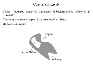
Cavity, concavity. Cavity – bounded connected component of background (a hollow in an object) Concavity - concave shapes of the contour of an object. 2D hole = 2D cavity. concavity. cavity, 2D hole. concavity. 3D hole and 3D cavity.

E N D
Cavity, concavity Cavity – bounded connected component of background (a hollow in an object) Concavity - concave shapes of the contour of an object. 2D hole = 2D cavity concavity cavity, 2D hole concavity
3D hole and 3D cavity There is no good precise mathematical definition of a 3D hole. There is only a method how we can detect a hole The presence of a hole in X is detected whenever there is a closed path in X that cannot be iteratively deformed in X to a single point. [Kong 89] According to the method a hole is not a subset of 3D space. [Coup 10a]
3D hole closing algorithm [Coup 10a]
3D hole closing algorithm [Coup 10a]
3D hole closing algorithm [Coup 10a]
3D hole closing algorithm [Coup 10a]
3D hole closing algorithm (i-th iteration) [Coup 10a]
3D hole closing algorithm (last but one iteration) Curve point (1D isthmus point) T = 2; Tb = 1 Surface points T = 1; Tb = 2 [Coup 10a]
3D hole closing algorithm Surface points T = 1; Tb = 2 [Coup 10a]
3D hole closing algorithm Let (Z3, m, n, B) is a digital image and Y is a rectangular prism set of black points such that B Y. The algorithm iteratively removes border points x of Y \ B such that Tb(x) = 1. The removing process is guided by a distance function of point x from set B. [Actouf 2002]
3D hole closing examples [Aktouf 02]
3D hole closing examples [Coup 10a]
3D selective closing of holes Input set: B, Y – rectangular prism: B Y The algorithm in addition deletes each point x which is a surface point (Tb(x) = 2 and T(x) = 1) and d(x, B) > a [Aktouf 02]
Properties of 3D hole closing algorithm • Linear in time and space (optimal). • Based on well defined topological characteristic of points. • No parameters to tune or only one parameter (size of a hole) when it utilises a distance map to close only small holes. • wide potential application (reparation of tomografic images, fast detection of holes). Drawbacks • Closes not only holes but also cavities. • Sensitive to branches which are close to a hole.
+ HCA which closes only holes
Skeletonisation HCO Geodezyjna dylacja Homotop. Skel. HCO with a new guide function Branches insensitive AZO
HCA+ HCA+ ( Input X, Output Z) 01. Xcf← CavitiesFilling(X) 02. Y ← HCA(Xcf) 03. Ydil← GeoDilat(Y;X) 04. C ← Ydil ∩ X 04. SC← UHS(C) 05. Z ← HCA(SC)
Filtered skeleton constrained by medial axis The algorithm uses the following notions: quadratic Euclidean distance, medial axis, Euclidean skeleton, bisector function. Denotes Let denote by E the discrete plane Z2,by N the set of nonnegative integers, and by N* the set of strictly positive integers. A point x in E is defined by (x1, x2) with xi in Z. Let x, y є E. Let denote by d2(x,y) the square of the Euclidean distance between x and y, that is, d2(x,y) = (x1, y1)2 + (x2 y2)2. Let Y E, let denote by d2(x,Y) the square of the Euclidean distance between x and the set Y, that is, d2(x,Y) = min{d2(x,y); yєY}.
Squared Euclidean distance map Let Xbe (the ‘‘object’’), we denote by themap from E to N which associates, to each point x of E,the value where denotes the complementaryof X (the ‘‘background’’). The map is called the (squared Euclidean) distance map of X.
t(y) y x t(x) Thickness of an object Let E = Z2 or E = R2, X E, and let x є X. The thickness t(x) of the object X at x is defined as a radius of a biggest ball among balls centred at x and included in X. [Atta 96]
c a y x b Projection Let X be a nonempty subset of E, andlet xєX.The projection of xon X, denoted by Pr(x,X), is the set ofpoints y of whichare at minimaldistance from x. [Coup 07]
c a y x θX(x) b Bisector function Let XE, and let xєX.The bisector angle of x in X, denoted by θX(x), is the maximalunsigned angle between the vectors ,, for all y,zin Pr(x, X). In particular, if #Pr(x, X) = 1, then θX(x) = 0. The bisector function of X, denoted by θX , is the functionwhich associates to each point x of X, its bisector angle in X.
c a x π y b d Bisector function in continuous space Let E = R2, X E, and let x є X. If x belongs to the medial axis of X, then its bisector angle is strictly positive. The bisector angle is equal to π for points where the thickness of the object is extremum [Vinc 91].
Extended projection Let E = Z2, XE and xєX. The extended projection of xonX, denoted by EPr(x, X), isthe union of thesets Pr(y;X), for all y in the 4-neighborhoodof x (6-neighborhood in Z3).
Extended bisector function Let XZ2, and let xєX.The extended bisector angle of x in X, denoted by, is the maximalunsigned angle between the vectors ,, for all y, zin EPr(x,X). The extended bisector function of X, denoted by, is the functionwhich associates to each point x of X, its extended bisector angle in X.
Niece-looking statement Let XZ2, and let xєX.If x belongs to the medial axis of X, then its extended bisector angle isstrictly positive. [Coup 07]
Using a bisector function for medial axis filtering in 2D [Coup 07]
Using extended bisector function for medial axis filtering in 3D Medial axis ExtendedBisector Filtered medial axis. Ext. Bis. Threshold: 2.7
Ultimate skeleton constrained by a set Let (E, m, n, B) be a digital image where E = Z2 lub Z3 and B is a finite subset of black points. Def of thinning is presented in slide 19. It is a process of iterative deletion of simple points form an input object B. We say that Y B is an ultimate skeleton of B if Y is an result of thinning of B and there is no simple point for Y. Let C be a subset of B. We say that Y is an ultimate skeleton of B constrained by C if the following conditions are true: • CY • Y is a result of thinning of B • there is no simple point in B \ C The set C is called the constraint set relative to this skeleton [Vinc 91].
Ultimate skeleton, constrained by a set and distance-guided Let C be a subset of B. We say that Y is an ultimate skeleton of Bconstrained by Cand distance-guided if Y is an ultimate skeleton of B constrained by C and the deletion of points is guided by a distance function d in order to select first the points which are closest to the background. UltimateGuidedSkeleton (Input B, d, C, Output Z) 01. Z←B 02. Q← {(d(x),x); where x is any point of B\ Y} 03. WhileQ≠θ; Do 04. choose (d(x),x) in Q such that d(x) is minimal 05. If x is simple for Z then 06. Z ← Z \ {x} 07.Q ← Q ∪ {(d(y), y); where y∊Nm(x) ∩ (Z \ Y)}
Filtered euclidean skeleton FilteredGuidedSkeleton (Input:B, r, , Output:Z) 01. DB←ExactSquaredEuclideanDistanceMap(B) 02. M←MedialAxis(X, DB ) 03. Θ←ExactBisector(M, DB ) 05. Y← {xєM;DB(x)≥r and Θ(x) ≥} 06. Z ←UltimateSkeleton(Z, DB, Y )
Example in 2D Non filtered filtered r = 0, = 2 filt. r = 64, = 2.2 filt. R=100, = 3.14 [Coup 07]
Example in 3D Medial axis Euclidean skeleton Filtered skeleton r = 1, = 1.5 [Coup 07]
Example in 3D r = 15; alfa = 1.5 [Coup 07]
References [Aktouf 02] Aktouf Z., Bertrand G., Perroton L.: A three-dimensional holes closing algorithm, Pattern Recognition Letters, vol. 23, pp. 523-31, 2002. [Alex 71] Alexander J. C., Thaler A. I., The boundary count of digital pictures, J Assoc. Comput Mach, pp. 105-112, 1971 [Atta 96] Attali D., Montanvert A., Modeling noise for a better simplification of skeletons, in Proc. of International Conference on Image Processing, 1996, pp. III: 13-16. [Coup 07] Couprie M., Coeurjolly D., Zrour R., Discrete bisector function and Euclidean skeleton in 2D and 3D, Image Vision Comput., vol. 25, pp. 1543-1556, 2007. [Coup 10] Michel Couprie’s webpage on simple points: http://www.esiee.fr/~info/ck/CK_simple.html [Coup 10a] Michel Couprie’s presentation on hole closing [Duda 67] Duda R. O., Hart P. E., H. M. J., Graphical-Data-Processing Research Study and Experimental Investigation, AD657670, 1967. [Hild 83] Hilditch C. J., Comparison of thinning algorithms on a parallel processor, Image Vision Comput, pp. 115-132, 1983. [Kong 89] Kong T. Y., A digital fundamental group, Computer Graphics, vol. 13, pp. 159-166, 1989. [Malan 10] George Malandain’s webpage on digital topology:http://wwwsop.inria.fr/epidaure/personnel/malandain/topology/ [Malina 02] Malina W., Ablameyko S., Pawlak W.: Podstawy cyfrowego przetwarzania obrazów, AOW Exit, 2002 (in polish) [Mylo 71] Mylopoulos J., Pavlidis T., On the topological properties of quantized spaces II: Connectivityand order of connectivity, J. Assoc. Comput. Mach, pp. 247-254, 1971. [Rose 70] Rosenfeld A., Connectivity in Digital Pictures, J. ACM, vol. 17, pp. 146-160, 1970. [Rose 73] Rosenfeld A., Ares and curves in digital pictures, J. Assoc. Comput. Mach. 20, 1973, 81 87. [Rose 86] Ronse C., A topological characterization of thinning, Theoret. Comput. Sci. 43, 1986, 31-41. [Stef 71] Stefanelli R., Rosenfeld A., Some parallel thinning algorithms for digital pictures, J. Assoc. Comput. Mach, pp. 255-264, 1971. [Vinc 91] Vincent L.: Efficient computation of varous types of skeletons. In SPIE’s Medical Imaging V, volume 1445, San Jose, CA, February 1991.