Download
1 / 42
450 likes | 633 Views
Learn about different types of boundary conditions in groundwater modeling, their implications, examples, and potential problems to avoid misunderstandings and ensure accurate simulations. This educational resource provides insights for researchers and practitioners.

E N D
Boundary Conditions Based on Slides Prepared By Eileen Poeter, Colorado School of Mines
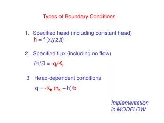
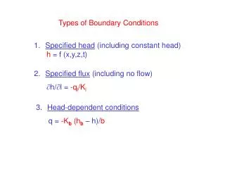
Types of Boundary Conditions 1) Specified Head: head is defined as a function of space and time (could replace ABC, EFG) Constant Head: a special case of specified head (ABC, EFG) 2) Specified Flow: could be recharge across (CD) or zero across (HI) No Flow (Streamline): a special case of specified flow where the flow is zero (HI) 3) Head Dependent Flow: could replace (ABC, EFG) Free Surface: water-table, phreatic surface (CD) Seepage Face: h = z; pressure = atmospheric at the ground surface (DE)
Three basic types of Boundary Conditions After: Definition of Boundary and Initial Conditions in the Analysis of Saturated Gournd-Water Flow Systems - An Introduction, O. Lehn Franke, Thomas E. Reilly, and Gordon D. Bennett, USGS - TWRI Chapter B5, Book 3, 1987.
DIRICHLETConstant Head & Specified Head Boundaries Specified Head: Head (H) is defined as a function of time and space. Constant Head: Head (H) is constant at a given location. Implications: Supply Inexhaustible, or Drainage Unfillable
Example: Constant Head Example of Potential Problems Which May Result From Misunderstanding / Misusing a Constant Head Boundary If heads are fixed at the ground surface to represent a swampy area,
Example: Constant Head and an open pit mine is simulated by defining heads in the pit area, to the elevation of the pit bottom,
Example: Constant Head the use of constant heads to represent the swamp will substantially overestimate in-flow to the pit. This is because the heads are inappropriately held high, while in the physical setting, the swamp would dry up and heads would decline, therefore actual in-flow would be lower. The swampy area is caused by a high water table. It is not an infinite source of water.
Example: Constant Head Lesson: Monitor the in-flow at constant head boundaries and make calculations to assure yourself the flow rates are reasonable.
Example: Specified Head Example of Potential Problems Which May Result From Misunderstanding / Misusing a Specified Head Boundary When a well is placed near a stream, and the stream is defined as a specified head,
Example: Specified Head the drawdown may be underestimated, if the pumping is large enough to affect the stream stage. The specified flow boundary may supply more water than the stream caries,
Example: Specified Head and drawdowns should be greater, for the given pumping rate. The stream stage, and flow rate, should decrease to reflect the impact of the pumping.
Example: Specified Head Lesson: Monitor the in-flow at specified head boundaries. Confirm that the flow is low enough relative to the streamflow, such that stream storage will not be affected.
NEUMANNNo Flow and Specified Flow Boundaries Specified Flow: Discharge (Q) varies with space and time. No Flow: Discharge (Q) equals 0.0 across boundary. Implications: H will be calculated as the value required to produce a gradient to yield that flow, given a specified hydraulic conductivity (K). The resulting head may be above the ground surface in an unconfined aquifer, or below the base of the aquifer where there is a pumping well; neither of these cases are desirable.
Example: SPECIFIED FLOW Example of Potential Problems Which May Result From Misunderstanding / Misusing a Specified Flow Boundary In this example, the model represents a simple unconfined aquifer with one well. Two cases are presented: 1) an injection well, and 2) a withdrawal (pumping) well.
Example: SPECIFIED FLOW Injection Well: If the injection flow is too large, calculated heads may be above the ground surface in unconfined aquifer models.
Example: SPECIFIED FLOW Withdrawal Well: If the withdrawal flow is too large, calculated heads may fall below the bottom of the aquifer, yet the model may still yield water.
Example: SPECIFIED FLOW Lesson: Monitor calculated heads at specified flow boundaries to ensure that the heads are physically reasonable.
Example: NO FLOW Example of Potential Problems Which May Result From Misunderstanding / Misusing a No Flow Boundary When a no flow boundary is used to represent a ground water divide, drawdown may be overestimated, and although the model does not indicate it, there may be impacts beyond the model boundaries.
Example: NO FLOW Simplified model with no-flow boundary representing the ground-water divide.
Example: NO FLOW Use of a no-flow boundary in this manner may cause problems: When a ground water divide is defined as a no-flow boundary, the flow system on the other side of the boundary cannot supply water to the well, therefore predicted drawdowns will be greater than would be experienced in the physical system. The no-flow boundary prevents the ground water divide from shifting, implying there drawdown is zero on the other side of the divide.
Example: NO FLOW Lesson: Monitor head at no flow boundaries used to represent flow lines or flow divides to ensure the location is valid even after the stress is applied.
CAUCHYHead Dependent Flow • Head Dependent Flow: • H1 = Specified head in reservoir • H2 = Head calculated in model • Implications: • If H2 is below AB, q is a constant and AB is the seepage face, but model may continue to calculate increased flow. • If H2 rises, H1 doesn't change in the model, but it may in the field. • If H2 is less than H1, and H1 rises in the physical setting, then inflow is underestimated. • If H2 is greater than H1, and H1 rises in the physical setting, then inflow is overestimated.
Free Surface Free Surface: h = Z, or H = f(Z) e.g. the water table h = z or a salt water interface Note, the position of the boundary is not fixed! Implications:Flow field geometry varies so transmissivity will vary with head (i.e., this is a nonlinear condition). If the water table is at the ground surface or higher, water should flow out of the model, as a spring or river, but the model design may not allow that to occur.
Seepage Surface Seepage Surface: The saturated zone intersects the ground surface at atmospheric pressure and water discharges as evaporation or as a downhill film of flow. The location of the surface is fixed, but its length varies (unknown a priori). Implications:A seepage surface is neither a head or flowline. Often seepage faces can be neglected in large scale models.
Natural and Artificial Boundaries It is most desirable to terminate your model at natural geohydrologic boundaries. However, we often need to limit the extent of the model in order to maintain the desired level of detail and still have the model execute in a reasonable amount of time. Consequently models sometimes have artificial boundaries. For example, heads may be fixed at known water table elevations at a county line, or a flowline or ground-water divide may be set as a no-flow boundary.
Boundary Condition Exercise Theis (many assumptions ) and Theim (radial flow to a well in confined conditions)
Boundary Condition Exercise Dupuit formula for radial flow under water table conditions
Boundary Condition Exercise Example: An oceanic island in a humid climate; permeable materials are underlain by relatively impermeable bedrock
Boundary Condition Exercise Example: An alluvial aquifer associated with a medium-sized river in a humid climate; the aquiferis underlain and bounded laterally by bedrock of low hydraulic conductivity
Boundary Condition Exercise Example: An alluvial aquifer associated with an intermittent stream in an arid climate; the aquifer is underlain and bounded laterally by bedrock of low to intermediate hydraulic conductivity
Boundary Condition Exercise Example: A western valley with internal drainage in an arid region; intermittent streams flow from surrounding mountains towards a valley floor; a part of valley floor is playa
Boundary Condition Exercise Example: A confined aquifer bounded above and below by leaky confining beds
Hydrologic Features as Boundaries • Boundary can be assigned to hydrologic feature such as: • Surface water body • Lake, river, or swamp • Water table • Recharge and evapotranspiration or source/sink specified head • Impermeable surface • Bedrock or permeable unit pinches out
Ground-water / Surface-water Interaction • Hydraulic head in aquifer can be equal to elevation of surface-water feature or allowed to leak to the surface-water feature • Usually defined as a “Constant-Head” or “Specified Head” Boundary or “Head-dependent flow” boundary • If elevation of SW changes, as with streams, elevation of the boundary condition changes
How a stream could interact with the ground-water system T.E. Reilly, 2000
South Carolina Well in the Piedmont Nearby stream gage correlates with well. (3) Source, Bruce Campbell, USGS, SC, 2000 Drought
No-Flow Boundary • Hydraulic conductivity contrasts between units • Alluvium on top of tight bedrock • Assume GW does not move across this boundary • Can use ground-water divide or flow line
Note ground-water divide shifts after development—may or may not be a good no-flow BC T.E. Reilly, 2000
Water Table or “Flow” Boundary • Intermittent areal recharge on water-table • Moves through unsaturated zone • Volume of water per unit area per unit of time entering the GW system is specified • May vary with time and space • Evapotranspiration occurs when plants remove water from the water-table • May be head-dependent (if water-table too far below land surface ET is unlikely • Volume of water per unit area per unit of time leaving the GW system as a function of depth to water is specified • May vary in space and time
Wells—an internal boundary condition at a point—thought of as a stress to the system • A well is a specified flow rate at a point • Can be pumping or injecting water • Withdrawals or injection may vary in space and time
Practical Considerations • Boundary conditions must be assigned to every point on the boundary surface • Modeled boundary conditions are usually greatly simplified compared to actual conditions