Download
1 / 17
170 likes | 297 Views
This study investigates the complex behavior of stars in the vicinity of the main sequence on the Hertzsprung-Russell diagram. It emphasizes the significance of pulsating stars as key indicators of evolutionary status, particularly distinguishing pre-main-sequence (PMS) from post-main-sequence (post-MS) stars. Utilizing seismological data, oscillatory frequency distributions are analyzed to enhance stellar classification. Key findings include the identification of specific pulsation characteristics in HAEBE stars. This work is supported by the Romanian Space Agency and contributes valuable insights into stellar evolution modeling.

E N D
Calibration of stellar evolution using stellar pulsations Marian Doru Suran, Nedelia Antonia Popescu Astronomical Institute of the Romanian Academy e-mail: suran@aira.astro.ro Supported by the Romanian Space Agency (ROSA) contract Nr. 124/30.09.2004
Abstract Close to the main sequence the HR diagram is confusing as stars of similar global properties but with different stages of evolution occupy the same position. Pulsating stars (both pms and post-ms) have been discovered in this area. In some cases the young pms stars are recognized through specific characteristics – for instance the presence of nebulosity or high degree of activity. An alternative is to take advantage of the seismological information whenever it is possible. In this case the discrimination between pms and post-ms can be made using differences in their oscillatory frequency distributions in the low frequency range.
Calibration method: • Stellar evolution: - CESAM vs. HENYEY(Bucharest); - 1.8M track (Figure 1, Table 2). • Evolutive pulsational diagram: - CESAM (osc.ad+nad) +LNANR (linear, nonadiabatic, nonradial, Suran, Bucharest); - 1.8M track(l=0-2, g,f,p,); - from pms post-ms (Figure 2a,b); - 3 common points (pms/post-ms): a.,b.,c, (see Figure 1 and Table 1).
Results - HAEBE stars: • Evolutive status: pms vs. post-ms: - V351 Ori (pt. c.) t [P=14.33 (f2), penetrative post-ms ?!] [BKW,C,M,RP] Table 3, Figure 3a,b. • Physical parameters: - V1366 Ori (pts. a.,d.,e.) Te [A] Table 4, Figure 4 a,b,c.
References: • Amado, P. J.; Moya, A.; Suárez, J. C.; Martín-Ruiz, S.; Garrido, R.; Rodríguez, E.; Catala, C.; Goupil, M. J., 2004, M.N.R.A.S.,352, pp. L11-L15 [A]; • Balona, L. A.; Koen, C.; van Wyk, F., 2003, M.N.R.A.S., 333, pp. 923-931 [BKW]; • Catala, C., 2003, Astrophysics and Space Science, pp. 53-60l [C] • Marconi, M.; Ripepi, V.; Palla, F.; Ruoppo, A., 2004, Communications in Asteroseismology, 145, pp. 61-66 [M]; • Ripepi, V.; Marconi, M.; Bernabei, S.; Palla, F.; Pinheiro, F. J. G.; Folha, D. F. M.; Oswalt, T. D.; Terranegra, L.; Arellano Ferro, A.; Jiang, X. J., 2003, Astronomy and Astrophysics, v.408, pp.1047-1055 (2003) [RP].
Table 1. Common pms and post-ms points on the track of 1.8M star.
Table 2. Physical data used in the models of V351 Ori and V1366 Ori
Figure 1. Evolutive tracks of 1.8 M star in the HRdiagram. [CESAM(C) vs. HENYEY(H)]. Common points pre/postMS labeled by a,b,c. In the figure also is indicated the main instability strip.
Figure 2.a. Evolutive pulsational diagram for a star of 1.8M[R] [l = 0 (square), l = 1 (*), l = 2 (+)]
Figure 2.b. Evolutive pulsational diagram for a star of 1.8M[I] . [l = 0 (square), l = 1 (*), l = 2 (+)]
Figure 3.a. Pulsational diagram for V351 Ori. Brown and light brown: observations (see table 3). Red and green (pms: l = 0,l = 2). Blue and magenta (post-ms: l = 0,l = 2).
Figura 4a. Pulsational diagram for V1366 Ori (point a.). Green points observations. Red and blue points: theoretical model [pms, point a., l = 0,l = 2] (see table 4)
Figura 4b. Pulsational diagram for V1366 Ori (point d.). Notations as in Figure 4a.
Figura 4c. Pulsational diagram for V1366 Ori (point e.). Notations as in Figure 4a.