Testing Hypotheses on Population Proportion Using Classical & p-Value Approaches
290 likes | 324 Views
Learn how to test hypotheses about population proportions using classical and p-value methods with practical examples and steps.

Testing Hypotheses on Population Proportion Using Classical & p-Value Approaches
E N D
Presentation Transcript
Testing Hypotheses about a Population Proportion Lecture 31 Sections 9.1 – 9.3 Wed, Mar 16, 2005
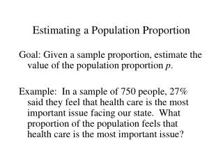
Discovering Characteristics of a Population • Any question about a population must first be described in terms of a population parameter. • Then the question about that parameter generally falls into one of two categories. • What is the value of the parameter? • That is, estimate its value. • Does the evidence support or refute a claim about the value of the parameter? • That is, test a hypothesis concerning the parameter.
Example • A standard assumption is that a newborn baby is as likely to be a boy as to be a girl. However, some people believe that boys are more likely. • Suppose a random sample of 1000 live births shows that 520 are boys and 480 are girls. • Use the data to estimate the proportion of male births. • Does this evidence support or refute the standard assumption?
Two Approaches for Hypothesis Testing • Classical approach. • Determine the critical value and the rejection region. • See whether the statistic falls in the rejection region. • Report the decision. • p-Value approach. • Compute the p-value of the statistic. • See whether the p-value is less than the significance level. • Report the p-value.
Classical Approach z c 0
Classical Approach z c 0 Rejection Region Acceptance Region
Classical Approach Reject z z c 0 Rejection Region Acceptance Region
Classical Approach Accept z z c 0 Rejection Region Acceptance Region
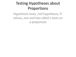
The Steps of Testing a Hypothesis (p-Value Approach) • The basic steps are • 1. State the null and alternative hypotheses. • 2. State the significance level. • 3. Compute the value of the test statistic. • 4. Compute the p-value. • 5. State the conclusion. • See page 519 (I omitted the first step.)
Step 1: State the Null and Alternative Hypotheses • Let p = proportion of live births that are boys. • The null and alternative hypotheses are • H0: p = 0.50. • H1: p > 0.50.
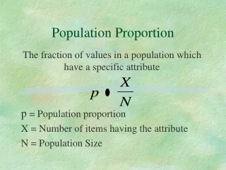
State the Null and Alternative Hypotheses • The null hypothesis should state a hypothetical value p0 for the population proportion. • H0: p = p0. • The alternative hypothesis must contradict the null hypothesis in one of three ways: • H1: p < p0. (Direction of extreme is left.) • H1: p p0. (Direction of extreme is left and right.) • H1: p > p0. (Direction of extreme is right.)
Explaining the Data • The observation is 520 males out of 1000 births, or 52%. That is, p^ = 0.52. • Since we did not observe 50%, how do we explain the discrepancy? • Chance, or • The true proportion is not 50%, but something larger, maybe 52%.
Step 2: State the Significance Level • The significance level should be given in the problem. • If it isn’t, then use = 0.05. • In this example, we will use = 0.05.
The Sampling Distribution of p^ • To decide whether the sample evidence is significant, we will compare the p-value to . • From the value of , we may find the critical value(s). • is the probability that the sample data are at least as extreme as the critical value(s), if the null hypothesis is true.
The Sampling Distribution of p^ • Therefore, when we compute the p-value, we do it under the assumption that H0 is true, i.e., that p = p0.
The Sampling Distribution of p^ • We know that the sampling distribution of p^ is normal with mean p and standard deviation • Thus, we assume that p^ has mean p0 and standard deviation:
Step 3: The Test Statistic • Test statistic – The z-score of p^, under the assumption that H0 is true. • Thus,
The Test Statistic • In our example, we compute • Therefore, the test statistic is • Now, to find the value of the test statistic, all we need to do is to collect the sample data and substitute the value of p^.
Computing the Test Statistic • In the sample, p^ = 0.52. • Thus, • z = (0.52 – 0.50)/0.0158 = 1.26.
Step 4: Compute the p-value • To compute the p-value, we must first check whether it is a one-tailed or a two-tailed test. • We will compute the probability that Z would be at least as extreme as the value of our test statistic. • If the test is two-tailed, then we must take into account both tails of the distribution to get the p-value.
Compute the p-value • In this example, the test is one-tailed, with the direction of extreme to the right. • So we compute P(Z > 1.26) = 0.1038.
Compute the p-value • An alternative is to evaluate normalcdf(0.52, E99, 0.50, 0.0158) on the TI-83. • It should give the same answer (except for round-off).
Step 5: State the Conclusion • Since the p-value is greater than , we should not reject the null hypothesis. • State the conclusion in a sentence. • “The data do not support the claim, at the 5% level of significance, that more than 50% of live births are male.”
Testing Hypotheses on the TI-83 • The TI-83 has special functions designed for hypothesis testing. • Press STAT. • Select the TESTS menu. • Select 1-PropZTest… • Press ENTER. • A window with several items appears.
Testing Hypotheses on the TI-83 • Enter the value of p0. Press ENTER and the down arrow. • Enter the numerator x of p^. Press ENTER and the down arrow. • Enter the sample size n. Press ENTER and the down arrow. • Select the type of alternative hypothesis. Press the down arrow. • Select Calculate. Press ENTER. • (You may select Draw to see a picture.)
Testing Hypotheses on the TI-83 • The display shows • The title “1-PropZTest” • The alternative hypothesis. • The value of the test statistic Z. • The p-value. • The value of p^. • The sample size. • We are interested in the p-value.