Download
1 / 36
370 likes | 453 Views
Rapid Protein Side-Chain Packing via Tree Decomposition. Jinbo Xu j3xu@tti-c.org Toyota Technological Institute at Chicago. Outline. Background Method Results. Biology in One Slide. organism. Protein. Proteins. Proteins are the building blocks of life.

E N D
Rapid Protein Side-Chain Packing via Tree Decomposition Jinbo Xu j3xu@tti-c.org Toyota Technological Institute at Chicago
Outline Background Method Results
Biology in One Slide organism Protein
Proteins Proteins are the building blocks of life. In a cell, 70% is water and 15%-20% are proteins. Examples: hormones – regulate metabolism structures – hair, wool, muscle,… antibodies – immune response enzymes – chemical reactions
Amino Acids A protein is composed of a central backbone and a collection of (typically) 50-2000 amino acids (a.k.a. residues). There are 20 different kinds of amino acids each consisting of up to 18 atoms, e.g., Name 3-letter code1-letter code Leucine Leu L Alanine Ala A Serine Ser S Glycine Gly G Valine Val V Glutamic acid Glu E Threonine Thr T
Protein Structure repeating backbone structure repeating backbone structure CH2 CH2 CH CH2 H C CH3 CH2 CH2 CH2 CH2 COO- CH2 H3CCH3 CH2 HC CH CH2 CH2 CH3 HN N OH NH CH C NH2 N+H2 AspArgValTyrIleHisProPhe DRVYIHP F Protein sequence: DRVYIHPF O H O H O H O H O H O H O H H3N+ CH C N CH C N CH C N CH C N CH C N CH C N CH C N CH COO-
Protein Structure Prediction • Stage 1: Backbone Prediction • Ab initio folding • Homology modeling • Protein threading • Stage 2: Loop Modeling • Stage 3: Side-Chain Packing • Stage 4: Structure Refinement The picture is adapted from http://www.cs.ucdavis.edu/~koehl/ProModel/fillgap.html
Protein Side-Chain Packing • Problem: given the backbone coordinates of a protein, predict the coordinates of the side-chain atoms • Insight: a protein structure is a geometric object with special features • Method: decompose a protein structure into some very small blocks What are their positions?
Torsion Angles Torsion angles of Lysine Each amino acid has 0 to 4 torsion angles. The positions of the side-chain atoms are determined if C-alpha, C-beta positions are known and torsion angles are fixed.
Conformation Discretization 0.2 0.167 0.167 clustering 0.1 0.133 0.1 0.133 The probabilities can depend on local backbone structures.
Side-Chain Packing 0.3 0.2 0.3 0.7 0.1 0.4 0.1 0.1 0.6 clash Each residue has many possible side-chain positions. Each possible position is called a rotamer. Need to avoid atomic clashes.
Energy Function Assume rotamer A(i) is assigned to residue i. The side-chain packing quality is measured by clash penalty 10 clash penalty 0.82 1 occurring preference The higher the occurring probability, the smaller the value : distance between two atoms :atom radii Minimize the energy function to obtain the best side-chain packing.
Related Work • NP-hard [Akutsu, 1997; Pierce et al., 2002] and NP-complete to achieve an approximation ratio O(N) [Chazelle et al, 2004] • Dead-End Elimination: eliminate rotamers one-by-one • Linear integer programming [Althaus et al, 2000; Eriksson et al, 2001; Kingsford et al, 2004] • Semidefinite programming [Chazelle et al, 2004] • SCWRL: biconnected decomposition of a protein structure [Dunbrack et al., 2003] • One of the most popular side-chain packing programs
Algorithm Overview • Model the potential atomic clash relationship using a residue interaction graph • Decompose a residue interaction graph into many small subgraphs (tree-decomposition) • Do side-chain packing to each subgraph almost independently
Residue Interaction Graph Each residue as a vertex Two residues interact if there is a potential clash between their rotamer atoms Add one edge between two residues that interact. h f b d s m c a e i j k l Residue Interaction Graph
Key Observations • A residue interaction graph is a geometric neighborhood graph • Each rotamer is bounded to its backbone by a constant distance • There is no interaction edge between two residues if their distance is beyond D. D is a constant depending on rotamer diameter. 2. A residue interaction graph is sparse! • Any two residue centers cannot be too close. Their distance is at least a constant C. No previous algorithms exploit these features!
h f d f abd b d g g m c m c a e i a e i j l k j k l Tree Decomposition[Robertson & Seymour, 1986] Greedy: minimum degree heuristic h • Choose the vertex with minimal degree • The chosen vertex and its neighbors form a component • Add one edge to any two neighbors of the chosen vertex • Remove the chosen vertex • Repeat the above steps until the graph is empty
h fgh f b d g m acd cdem defm abd c a e i clk eij remove dem j k l fgh ab ac c f clk ij Tree Decomposition (Cont’d) Tree Decomposition Tree width is the maximal component size minus 1.
Xir Xr Xi Xp Xli Xji Xq Xj Xl Side-Chain Packing Algorithm 1. Bottom-to-Top: Calculate the minimal energy function 2. Top-to-Bottom: Extract the optimal assignment 3. Time complexity: exponential to tree width, linear to graph size A tree decomposition rooted at Xr The score of component Xi The scores of subtree rooted at Xl The score of subtree rooted at Xi The scores of subtree rooted at Xj
Theoretical Treewidth Bounds • For a general graph, it is NP-hard to determine its optimal treewidth. • Has a treewidth • Can be found within a low-degree polynomial-time algorithm, based on Sphere Separator Theorem [G.L. Miller et al., 1997], a generalization of the Planar Separator Theorem • Has a treewidth lower bound • The residue interaction graph is a cube • Each residue is a grid point
Sphere Separator Theorem [G.L. Miller & S.H. Teng et al, 1997] • K-ply neighborhood system • A set of balls in three dimensional space • No point is within more than k balls • Sphere separator theorem • If N balls form a k-ply system, then there is a sphere separator S such that • At most 4N/5 balls are totally inside S • At most 4N/5 balls are totally outside S • At most balls intersect S • S can be calculated in random linear time
D Residue Interaction Graph Separator • Construct a ball with radius D/2 centered at each residue • All the balls form a k-ply neighborhood system. k is a constant depending on D and C. • All the residues in the blue cycles form a balanced separator with size .
Height= Separator-Based Decomposition S1 S2 S3 S4 S5 S6 S7 S9 S12 S8 S10 S11 • Each Si is a separator with size • Each Si corresponds to a component • All the separators on a path from Si to S1 form a tree decomposition component.
Empirical Component Size Distribution DEE is conducted before tree decomposition. Otherwise, component size will be bigger. Tested on the 180 proteins used by SCWRL 3.0. Components with size ≤ 2 ignored.
Result (1) Theoretical time complexity: << is the average number rotamers for each residue. Five times faster on average, tested on 180 proteins used by SCWRL 3.0 Same prediction accuracy as SCWRL CPU time (seconds) TreePack can solve some instances that SCWRL cannot!!!
Result (2): Chi1 Accuracy A prediction is judged correct if its deviation from the experimental value is within 40 degree.
Result (3): Non-native Backbones Tested on 24 CASP6 targets, backbone structures are generated by RAPTOR+MODLLER.
Result (4) An optimization problem admits a PTAS if given an error ε (0<ε<1), there is a polynomial-time algorithm to obtain a solution close to the optimal within a factor of (1±ε). • Has a PTAS if one of the following conditions is satisfied: • All the energy items are non-positive • All the pairwise energy items have the same sign, and the lowest system energy is away from 0 by a certain amount Chazelle et al. have proved that it is NP-complete to approximate this problem within a factor of O(N), without considering the geometric characteristics of a protein structure.
A PTAS for Side-Chain Packing kD kD kD D D … Tree width O(1) Tree width O(k) Partition the residue interaction graph to two parts and do side-chain assignment separately.
A PTAS (Cont’d) To obtain a good solution • Cycle-shift the shadowed area by iD (i=1, 2, …, k-1) units to obtain k different partition schemes • At least one partition scheme can generate a good side-chain assignment
Cryo-EM density map of the gap junction channel, at 5.7 Å resolution in the membrane plane and 19.8 Å resolution in the vertical direction. The alpha-carbon model presented in Fleishman et. al., Molecular Cell15, 879–888 (2004) is superimposed. Red spheres, corresponding to disease-causing mutations, are located at helix-helix interfaces. Cryo-EM density map of the gap junction channel, at 5.7 Å resolution in the membrane plane and 19.8 Å resolution in the vertical direction. The alpha-carbon model presented in Fleishman et. al., Molecular Cell15, 879–888 (2004) is superimposed. Red spheres, corresponding to disease-causing mutations, are located at helix-helix interfaces. Cryo-EM density map of the gap junction channel, at 5.7 Å resolution in the membrane plane and 19.8 Å resolution in the vertical direction. The alpha-carbon model presented in Fleishman et. al., Molecular Cell15, 879–888 (2004) is superimposed. Red spheres, corresponding to disease-causing mutations, are located at helix-helix interfaces. Cryo-EM density map of the gap junction channel, at 5.7 Å resolution in the membrane plane and 19.8 Å resolution in the vertical direction. The alpha-carbon model presented in Fleishman et. al., Molecular Cell15, 879–888 (2004) is superimposed. Red spheres, corresponding to disease-causing mutations, are located at helix-helix interfaces. Cryo-EM density map of the gap junction channel, at 5.7 Å resolution in the membrane plane and 19.8 Å resolution in the vertical direction. The alpha-carbon model presented in Fleishman et. al., Molecular Cell15, 879–888 (2004) is superimposed. Red spheres, corresponding to disease-causing mutations, are located at helix-helix interfaces. Cryo-EM density map of the gap junction channel, at 5.7 Å resolution in the membrane plane and 19.8 Å resolution in the vertical direction. The alpha-carbon model presented in Fleishman et. al., Molecular Cell15, 879–888 (2004) is superimposed. Red spheres, corresponding to disease-causing mutations, are located at helix-helix interfaces. 1” 1” 1” 1” 1’ 1’ 1’ 1’ 1 1 1 1 3’ 3’ 3’ 3’ 2 2 2 2 3 3 3 3 2’ 2’ 2’ 2’ 2” 2” 2” 2” 3” 3” 3” 3” 4” 4” 4” 4” 4’ 4’ 4’ 4’ 4 4 4 4 Half of the connexon model has been cropped to view the side chain packing between the various helices. The coloring is by polarity, as in the CPK figure. Most aromatic side chains are packed between the putative 4-helix bundles, as well as on the perimeter facing the lipid. Application to Membrane Proteins RMSD=5.7Å RMSD=19.8Å RMSD=0.6Å Pictures are taken from Julio Kovacs. Cryo-EM density map of the gap junction channel, at 5.7 Å resolution in the membrane plane and 19.8 Å resolution in the vertical direction. The alpha-carbon model presented in Fleishman et. al., Molecular Cell15, 879–888 (2004) is superimposed. Red spheres, corresponding to disease-causing mutations, are located at helix-helix interfaces. Cryo-EM density map of the gap junction channel, at 5.7 Å resolution in the membrane plane and 19.8 Å resolution in the vertical direction. The alpha-carbon model presented in Fleishman et. al., Molecular Cell15, 879–888 (2004) is superimposed. Red spheres, corresponding to disease-causing mutations, are located at helix-helix interfaces.
Summary Give a novel tree-decomposition-based algorithm for protein side-chain prediction • Exploit the geometric features of a protein structure • Theoretical bound of time complexity • Polynomial-time approximation scheme • Efficient in practice, good accuracy • Can be used for sampling-based ab intio protein folding Work To Do • Add more energy items to the energy function • Apply the algorithm to protein docking and protein interaction prediction TreePack at http://ttic.uchicago.edu/~jinbo/TreePack.htm
Acknowledgements Ming Li (Waterloo) Bonnie Berger (MIT)
h f d abd g m c a h e i f b d j l k g m c a e i j k l Original Graph Tree Decomposition[Robertson & Seymour, 1986] Greedy: minimum degree heuristic h f d g abd acd m c e i j l k
Tree Decomposition[Robertson & Seymour, 1986] • Let G=(V,E) be a graph. A tree decomposition (T, X) satisfies the following conditions. • T=(I, F) is a tree with node set I and edge set F • Each element in X is a subset of V and is also a component in the tree decomposition. Union of all elements is equal to V. • There is an one-to-one mapping between I and X • For any edge (v,w) in E, there is at least one X(i) in X such that v and w are in X(i) • In tree T, if node j is a node on the path from i to k, then the intersection between X(i) and X(k) is a subset of X(j) • Tree width is defined to be the maximal component size minus 1