INTRODUCTION TO MICROECONOMICS

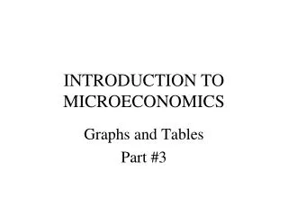
INTRODUCTION TO MICROECONOMICS Graphs and Tables Part #1

Figure II-1.1: The Increased Coordination of Decentralized Decision-makers’ Plans Producers (make plans) Error Correction P decrease Produce too much Consume too little Error Correction P increase Produce too little Consume too much Consumers (make plans)

Figure II-1.2: Basic Structure of a Market COMPETITION PRODUCERS COOPERATION COOPERATION CONSUMERS COMPETITION

Table II-2: Demand Schedule for Gasoline

Figure II-2: Demand Curve for Gasoline P $6 $5 $4 D Q 50 100

Table II-3: Supply Schedule for Gasoline

Figure II-3: Supply Curve of Gasoline S P $3 $2 $1 Q 50 100

Table II-4: The Market for Gasoline--Supply and Demand Schedules Combined

Figure II-4.1: The Market for Gasoline--Supply and Demand Curves P S $6.00 $3.50 D $1.00 Q 125

Figure II-4.2: Excess Supply of Gasoline P S $6.00 ES $4.50 $3.50 D $1.00 Q 125 175 75 ES = QS - QD =

Figure II-4.2a: Excess Supply of Gasoline P S $6.00 ES $4.50 $4.00 $3.50 D $1.00 Q 125 175 75 At P = $4, ES =

FigureII-4.3: Excess Demand for Gasoline P S $6.00 $3.50 $2.50 ED D $1.00 Q 175 75 125 ED = QD - QS=

FigureII-4.3a: Excess Demand for Gasoline P S $6.00 $3.50 $3.00 $2.50 ED D $1.00 Q 175 75 125 When P = $3.00, ED =

Table II-5a: An Increase in Demand, QD1

Figure II-5.1: An Increase in Demand P $7.00 $6.00 D1 $3.50 D0 Q 175 125 (1) An Increase in Demand (2) An Increase in the Quantity Demanded At Each Price

Table II-5b: A Decrease in Demand, QD2

Figure II-5.2: An Increase in the Quantity Demanded P $6.00 $3.50 1 $2.50 D0 Q 125 175 2 A Movement Along a Given Demand Curve

Table II-5c: Summary of a Crucial Distinction

Table II-5a: An Increase in Demand, QD1

Figure II-5.3: The Market for Gasoline Showing An Increase in Demand P $7.00 S $6.00 $4.00 $3.50 D1 D0 $1.00 Q 150 125

Table II-6a: An Increase in Supply, QS1

Figure II-6.1: An Increase in Supply P S0 S1 $3.50 $1.00 $0.00 Q 125 175 (1) Increase in Supply (2) Increase in the Quantity Supplied At Each Price

Table II-6b: A Decrease in Supply, QS2

Figure II-6.2: An Increase in the Quantity Supplied S0 P $4.50 1 $3.50 $1.00 Q 125 175 2 A Movement Along a Given Supply Curve

Table II-6c: Summary of a Crucial Distinction

Table II-6a: An Increase in Supply, QS1

Figure II-6.3:The Market for Gasoline Showing An Increase in Supply P S0 S1 $6.00 $3.50 $3.00 $1.00 D Q $0.00 125 150

Figure II-7: Selling Tickets and Scalping P S $100 $50 D1 D0 Q 5,000 10,000 20,000 D0 = Regular Event Demand Curve D1 = Very Popular Event Demand Curve

Table II-8: The Market for Bicycles

Figure II-8.1: A Consumer’s Surplus P S $120 CS $95 $70 D $20 Q 500 1000 CS for the 500th unit = $95 - $70 = $25 Consumer gains from trade for 500th unit.

Figure II-8.2: Consumers’ Surplus (CS) P S CS $120 $70 D $20 Q 1000 CS = 1/2 bh = 1/2(1,000)($120 - $70) = $25,000 = Total consumer gains from trade

Figure II-8.3: A Producer’s Surplus P S $120 $70 $45 PS D $20 Q 500 1,000 PS for the 500th unit = $70 - $45 = $25 Producer gains from trade for 500th unit

Figure II-8.4: Producers’ Surplus (PS) P S $120 $70 $45 D PS $20 Q 500 1,000 PS = ½ (b)(h) = ½ (1000)($70 - $20) = $25,000 = Total Producer Gains from Trade

Figure II-9: The Social Welfare Maximum P S $120 CS = $25,000 $70 D PS = $25,000 $20 Q 1,000 Note: (1) The Gains from Trade are Maximized at the Social Welfare Maximum. (2) CS + PS = $50,000

Table II-10a: Imposing Taxes on Producers

How to Adjust the Supply Schedule for a Tax • 1. Choose any quantity supplied (QS) from the supply schedule, say 1,200. • 2. The minimum price associated with supplying the 1,200th unit is $80. • 3. Since imposing a tax increases the costs of production for a producer, we should add the tax of $20 to the price of $80, yielding $100 as the minimum price at which a producer is willing and able to produce the 1,200th unit. • 4. The rest of the numbers for the new supply schedule can be filled in noting that every $10 change in price yields a 200 unit change in the quantity supplied. • 5. We now have a new supply schedule which represents a decrease in supply

Figure II-10.1: The Effect of a Tax on the Supply Curve P STAX = $20 $100 S0 $80 $40 $20 Q 1,200 Note that the tax causes a decrease in supply

Figure II-10.2: The Effect of a Tax on a Market P STAX=$20 CS’ S0 $120 P1 = $80 WL P0 = $70 TaxRev P2 = $60 $40 D PS’ $20 Q Q1 = 800 1,000 = Q0

Steps for Understanding How a Tax on Producers Affects the Market and Causes a Welfare Loss • 1. Social Welfare Maximum, Original Equilibrium, P = $70, Q = 1,000 • 2. Impose a Tax = $20, Decrease Supply • 3. New Equilibrium, P = $80, Q = 800 • 4. New CS’ = ½ (800)($120-$80) = $16,000 • 5. New PS’ = ½ (800)($60-$20) = $16,000 • 6. Tax Rev = (800)($20) = $16,000 • 7. Compare Before and After Tax CS and PS • CS + PS = $50,000 • CS’ + PS’ + Tax Rev = $48,000 • 8. WL = ½ ($20)(200) = $2,000

Figure II-10.3: Effect of a Producer Tax • Tax on producers results in misallocation of resources: Too little output in Taxed Market and too much output in the Rest of Economy Producer Tax Rest of Economy Market Resources (Lower Valued Uses) Output Decreases Output Increases Producer Tax on Market is equivalent to a subsidy for the Rest of Economy

Table II-10b: Imposing Taxes on Producers

Figure II-10.4: The Effect of a Tax on the Supply Curve P S0 $10 $2 Q

Figure II-10.5: The Effect of a Tax on the Supply Curve P S0 $22 $12 D $2 Q 5,000

Table II-11: Granting a Subsidy to Producers

How to Adjust the Supply Schedule for a Subsidy • 1. Choose any quantity supplied (QS) from the supply schedule. Say 1,200. • 2. The minimum price associated with supplying the 1,200th unit is $80. • 3. Since granting a subsidy decreases the costs of production for a producer, we should subtract the subsidy of $20 from the price of $80, yielding $60 as the minimum price that a producer is willing and able to produce the 1,200th unit. • 4.The rest of the numbers for the new supply schedule can be filled in noting that every $10 change in price yields a 200 unit change in the quantity supplied. • 5. We now have a new supply schedule which represents an increase in supply

Figure II-11.1: The Effect of a Subsidy on the Supply Curve S0 P SSUB=$20 $80 $60 $20 Q $00 1,200 Note that the subsidy causes an increase in supply.

Figure II-11.2: The Welfare Loss from a Subsidy to Producers S0 P $120 SSUB=$20 P2 = $80 P0 = $70 WL P1 = $60 $20 D $00 Q 1,200 = Q1 Q0 = 1,000

Steps for Understanding How a Subsidy to Producers Affects the Market and Causes a Welfare Loss • 1. Social Welfare Maximum, Original Equilibrium, P = $70, Q = 1,000 • 2. Grant a Subsidy = $20, Increase Supply • 3. New Equilibrium, P = $60, Q = 1,200 • 4. Total Subsidy = (1,200)($20) = $24,000 • 5. WL = $2,000 = ½ ($20)(200)

Figure II-11.3: Effect of a Producer Subsidy • Subsidy to producers results in misallocation of resources: Too much output in subsidized Market and too little output in the Rest of Economy Producer Subsidy Rest of Economy Market Resources (Lower Valued Use) Output Increases Output Decrease s Producer Subsidy in Market is equivalent to a tax on the Rest of Economy

Table II-12: The Market for Rental Housing

INTRODUCTION TO MICROECONOMICS