Download
1 / 27
1k likes | 4.05k Views
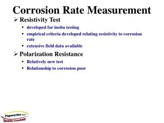
6. Corrosion Rate Measurements. 6.1 Weight loss measurement Specimen preparation Exposure to environment Specimen cleaning Measurement of change in specimen weight. • Corrosion rate expressions. - mm/y : mm penetration per year. - gmd : grams/m2 day

E N D
6. Corrosion Rate Measurements 6.1 Weight loss measurementSpecimen preparation Exposure to environment Specimen cleaning Measurement of change in specimen weight. • Corrosion rate expressions.- mm/y : mm penetration per year. - gmd : grams/m2 day - ipy : inches penetration per year - mpy : milli-inches per year - mdd : mg per square decimeter per day.i) corr. rate < 0.15 mm/y : good corrosion resistance for critical parts.ii) 0.15 < corr. rate < 1.5 mm/y : satisfactory if higher rate of corrosion can be tolerated, for example; tanks, piping and bolt heads.iii) corr. rate > 1.5 mm/y : usually not satisfactory.[ HOME WORK] 1) Prove that : mpy = 534W/DAT where, W= weight loss, mg. D= density of specimen A = area of specimen, inch2T = exposure time, hr 2) A piece of iron is observed to exhibit a uniform corrosion rate of 10 mdd. What is the corrosion current density in A/cm2 ?
6.2 Electrochemical Method - Based on the mixed potential theory.1) Tafel extrapolation Corrosion rate is determined by extrapolation of Tafel region to the corrosion potential. io,H2 on metal M is also determined by the intersection of the Tafel line with the reversible hydrogen potential. • Disadvantage of Tafel extrapolation method - only applied to systems containing one reduction process - interferences from conc. polarization in determining Tafel region.
E E' ic ia Ecorr io,a log i 2) Linear polarization method Within 10mV more noble or active than the Ecorr, ie is a linear function of the electrode potential. ie = I ia - ic I = f(E) E = E' - Ecorr = Ba log ia/io,M - Ba log icorr/io,M = Ba log ia/icorr = Ba/2.3 ln ia/icorr ia = icorr e2.3E/Ba Similarly, ic = icorr e-2.3E/Bc ie = ia - ic = icorr ( e2.3E/Ba– e-2.3E/Bc) = icorr (2.3E/Ba + 2.3E/Bc ) = 2.3icorrE(Ba + Bc)/BaBc Stern Geary eq. assuming that Ba = Bc = 0.12 Rp = E/ie = 0.026/icorrRp : polarization resistance.
6.3 Application of Impedance Technique on Corrosion Research • Electrochemical impedance spectroscopy (EIS) • The response of corroding electrodes to small-amplitude alternating potential signals of widely varying frequency has been analyzed by EIS. • v ( t ) = Vm sin ( wt )i ( t )= Im sin ( wt + ) • Why EIS ? • - In-situ : electrical properties of the interface between electrode and • electrolyte. • - Nondestructive : using very small amplitude signals.
The Double Layer The adsorbed fixed layer and the diffuse mobile layer together are the ELECTROCHEMICAL DOUBLE LAYER acting as a capacitor.
DC & The Double Layer • Surface atoms ionize and the electron flow towards the dc power supply. : " Faradaic Current " • The distance between the mobile layer and the electrode depends on dc voltage. DC voltage makes a net current flow through the double layer, from plate to plate, The double layer capacitor 'leaks'.
Behavior of The Double Layer With AC, The double layer behaves like a capacitor (Cdl)With DC, The double layer behaves like a resistor, The Faradaic resistor, (Rf)
AC & DC Behavior of The Double Layer With low frequency, Cdl is high. ⇒ current through Re (electrolyte resistor) and Rf, dc behavior rules. With high frequency, Cdl is low. ⇒ current through Cdl, ac behavior rules
Resistive Circuit eR eR • : angular frequency • = 2 No Phase difference between. eR and iR ER
: capacitive reactance Define Capacitive Circuit ec ec ec Ec 90° Phase difference between. ec and ic
rotating at same frequency I : phasor of the current, i E : phasor of the voltage, e : phase angle • • Phasor Diagram rotating vector (or phasor) phasor diagram e = E sin t radius : amplitude E frequency of rotation : e = E sin t i = I sin ( t -Φ)
• • • E I I • • I = E/R E = I R • • Resistive Circuit e e = E sin t i = (E/R) sin t (Ohm’s law) phasor notation Capacitive Circuit Re e • • Im E = -j XcI e = E sin t i = CE cos t = (E/Xc) sin( t +/2 ) • • E = -j XcI
• • • E = ER +EC E = I ( R – jXC) E = I Z R • • • • iR = I e iC = I C AC Voltage & Current Relation of the R-C circuit Z = R –jXC Z() = ZRe–jZIm • • • R ER = I R I • • -j Xc • • EC = -j XcI E = I Z Z
Nyquist Plot & Bode Plot The variation of the impedance with frequency can be displayed in different way. 1) Nyquist plot : displays ZIm vs. ZRe for different values of 2) Bode plot : log |Z| and are both plotted against log
R iR = I iC = I C High frequency : Z = R Low frequency : Z = Series Connection of the R-C Circuit ZRe= R , ZIm = -1/(wC) ( Xc : capacitive reactance ) -ZIm Z(w) Xc tan = ZIm/ZRe = Xc/R = 1/RC R ZRe
Series Connection of the R-C Circuit low freq. |Z| = 100 10-4 F High freq. |Z| = 0 ZIm w low freq. = -90 o High freq. = 0 o ZRe
High frequency : Z = 0 Low frequency : Z = R Parallel Connection of the R-C Circuit , w ZIm R ZRe
Parallel Connection of the R-C Circuit 100 |Z| = R 10-4 F |Z| = 0 w ZIm = -90 o = 0 o ZRe R
Randle Circuit Rs : solution resistance Rct : charge transfer resistance Cdl : double layer capacitance w ZIm , High frequency : Z = Rs Low frequency : Z = Rs+Rct Rs Rs+Rct ZRe
Randle Circuit 10-4 F 10 Rs+Rct 100 Rs wmax = 100 = 2, = 100/(2) 16 Hz wmax=1/(RctCdl) max -Rct/2 high freq. max Rs Rs+Rct/2 Rs+Rct
slope=1 High freq. : W = 0 Low freq. : W = Full Randle Circuit • Warburg impedance, W • diffusion control reaction • Usually observed in low frequency region : Warburg impedance coefficient R : ideal gas constant T : absolute temperature n : the number of electron transferred F : Faraday’s constant Cox : conc. of oxidation species Cred : conc. of reduction species Dox : diffusivity of oxidation species Dred : diffusivity of reduction species w Rs Rs+Rct
Full Randle Circuit w Nyquist plot Bode plot
Pore Rs Solution Rpo Cc Coating Rct Cdl Metal Equivalent Circuit of the Porous Coating Bode plot log |z| Rct Rpo Rs Cc Rpo Rct Cdl : solution resistance : capacitance of the coating : resistance of the porous layer : charge transfer resistance : double layer capacitance log freq.