The Underlying Event in Hard Scattering Processes
440 likes | 578 Views
The Underlying Event in Hard Scattering Processes. The Underlying Event : beam-beam remnants initial-state radiation multiple-parton interactions.

The Underlying Event in Hard Scattering Processes
E N D
Presentation Transcript
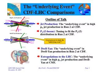
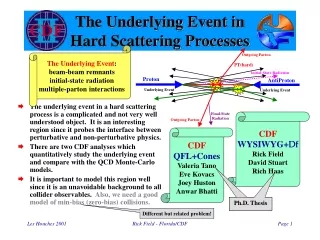
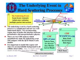
The Underlying Event inHard Scattering Processes The Underlying Event: beam-beam remnants initial-state radiation multiple-parton interactions • The underlying event in a hard scattering process is a complicated and not very well understood object. It is an interesting region since it probes the interface between perturbative and non-perturbative physics. • There are two CDF analyses which quantitatively study the underlying event and compare with the QCD Monte-Carlo models. • It is important to model this region well since it is an unavoidable background to all collider observables. Also, we need a good model of min-bias (zero-bias) collisions. CDF WYSIWYG+Df Rick Field David Stuart Rich Haas CDF QFL+Cones Valeria Tano Eve Kovacs Joey Huston Anwar Bhatti Ph.D. Thesis Ph.D. Thesis Different but related problem! Rick Field - Florida/CDF
Beam-Beam Remnants • The underlying event in a hard scattering process has a “hard” component (particles that arise from initial & final-state radiation and from the outgoing hard scattered partons) and a “soft” component (beam-beam remnants). • However the “soft” component is color connected to the “hard” component so this separation is (at best) an approximation. Min-Bias? • For ISAJET (no color flow) the “soft” and “hard” components are completely independent and the model for the beam-beam remnant component is the same as for min-bias (“cut pomeron”) but with a larger <PT>. • HERWIG breaks the color connection with a soft q-qbar pair and then models the beam-beam remnant component the same as HERWIG min-bias (cluster decay). Rick Field - Florida/CDF
Multiple Parton Interactions • PYTHIA models the “soft” component of the underlying event with color string fragmentation, but in addition includes a contribution arising from multiple parton interactions (MPI) in which one interaction is hard and the other is “semi-hard”. • The probability that a hard scattering events also contains a semi-hard multiple parton interaction can be varied but adjusting the cut-off for the MPI. • One can also adjust whether the probability of a MPI depends on the PT of the hard scattering, PT(hard) (constant cross section or varying with impact parameter). • One can adjust the color connections and flavor of the MPI (singlet or nearest neighbor, q-qbar or glue-glue). • Also, one can adjust how the probability of a MPI depends on PT(hard) (single or double Gaussian matter distribution). Rick Field - Florida/CDF
WYSIWYG: Comparing Datawith QCD Monte-Carlo Models Charged Particle Data QCD Monte-Carlo WYSIWYG What you see is what you get. Almost! • Zero or one vertex • |zc-zv| < 2 cm, |CTC d0| < 1 cm • Require PT > 0.5 GeV, |h| < 1 • Assume a uniform track finding efficiency of 92% • Errors include both statistical and correlated systematic uncertainties Select “clean” region Make efficiency corrections Look only at the charged particles measured by the CTC. • Require PT > 0.5 GeV, |h| < 1 • Make an 8% correction for the track finding efficiency • Errors (statistical plus systematic) of around 5% compare Small Corrections! Corrected theory Uncorrected data Rick Field - Florida/CDF
Charged Particle DfCorrelations • Look at charged particle correlations in the azimuthal angle Df relative to the leading charged particle jet. • Define |Df| < 60o as “Toward”, 60o < |Df| < 120o as “Transverse”, and |Df| > 120o as “Away”. • All three regions have the same size in h-f space, DhxDf = 2x120o = 4p/3. Rick Field - Florida/CDF
Charged Multiplicity versus PT(chgjet#1) • Data on the average number of “toward” (|Df|<60o), “transverse” (60<|Df|<120o), and “away” (|Df|>120o) charged particles (PT > 0.5 GeV, |h| < 1, including jet#1) as a function of the transverse momentum of the leading charged particle jet. Each point corresponds to the <Nchg> in a 1 GeV bin. The solid (open) points are the Min-Bias (JET20) data. The errors on the (uncorrected) data include both statistical and correlated systematic uncertainties. Underlying Event “plateau” Rick Field - Florida/CDF
Shape of an AverageEvent with PT(chgjet#1) = 20 GeV/c Includes Jet#1 Underlying event “plateau” Remember |h| < 1 PT > 0.5 GeV Shape in Nchg Rick Field - Florida/CDF
“Height” of the UnderlyingEvent “Plateau” Implies 1.09*3(2.4)/2 = 3.9 charged particles per unit h with PT > 0.5 GeV/c. Hard Soft 4 per unit h Implies 2.3*3.9 = 9 charged particles per unit h with PT > 0 GeV/c which is a factor of 2 larger than “soft” collisions. Rick Field - Florida/CDF
“Transverse” PT Distribution • Plot shows the PT distribution of the “Transverse” <Nchg>, dNchg/dPT. The integral of dNchg/dPT is the “Transverse” <Nchg>. • The triangle and circle (square) points are the Min-Bias (JET20) data. The errors on the (uncorrected) data include both statistical and correlated systematic uncertainties. Rick Field - Florida/CDF
“Transverse” PT Distribution • Comparison of the “transverse” <Nchg> versus PT(charged jet#1) with the PT distribution of the “transverse” <Nchg>, dNchg/dPT. The integral of dNchg/dPT is the “transverse” <Nchg>. Shows how the “transverse” <Nchg> is distributed in PT. PT(charged jet#1) > 30 GeV/c “Transverse” <Nchg> = 2.3 PT(charged jet#1) > 5 GeV/c “Transverse” <Nchg> = 2.2 Rick Field - Florida/CDF
“Max/Min Transverse” Nchg versus PT(chgjet#1) • Define “TransMAX” and “TransMIN” to be the maximum and minimum of the region 60o<Df<120o (60o<-Df<120o) on an event by event basis. The overall “transverse” region is the sum of “TransMAX” and “TransMIN”. The plot shows the average “TransMAX” Nchg and “TransMIN” Nchg versus PT(charged jet#1). • The solid (open) points are the Min-Bias (JET20) data. The errors on the (uncorrected) data include both statistical and correlated systematic uncertainties. Area DhDf 2x60o = 2p/3 “TransMAX” “TransMIN” Rick Field - Florida/CDF
“TransSUM/DIF” Nchg versus PT(chgjet#1) • Define “TransMAX” and “TransMIN” to be the maximum and minimum of the region 60o<Df<120o (60o<-Df<120o) on an event by event basis. The plot shows the average sum and difference of the “TransMAX” Nchg and the “TransMIN” Nchg versus PT(charged jet#1). The overall “transverse” region is the sum of “TransMAX” and “TransMIN”. • The solid (open) points are the Min-Bias (JET20) data. The errors on the (uncorrected) data include both statistical and correlated systematic uncertainties. Area DhDf 2x60o = 2p/3 “TransSUM” “TransDIF” Rick Field - Florida/CDF
“Max/Min Transverse” PTsum versus PT(chgjet#1) • Define “TransMAX” and “TransMIN” to be the maximum and minimum of the region 60o<Df<120o (60o<-Df<120o) on an event by event basis. The overall “transverse” region is the sum of “TransMAX” and “TransMIN”. The plot shows the average “TransMAX” PTsum and “TransMIN” PTsum versus PT(charged jet#1).. • The solid (open) points are the Min-Bias (JET20) data. The errors on the (uncorrected) data include both statistical and correlated systematic uncertainties. Area DhDf 2x60o = 2p/3 “TransMAX” “TransMIN” Rick Field - Florida/CDF
“TransSUM/DIF” PTsum versus PT(chgjet#1) • Define “TransMAX” and “TransMIN” to be the maximum and minimum of the region 60o<Df<120o (60o<-Df<120o) on an event by event basis. The plot shows the average sum and difference of the “TransMAX” PTsum and the “TransMIN” PTsum versus PT(charged jet#1). The overall “transverse” region is the sum of “TransMAX” and “TransMIN”. • The solid (open) points are the Min-Bias (JET20) data. The errors on the (uncorrected) data include both statistical and correlated systematic uncertainties. Area DhDf 2x60o = 2p/3 “TransSUM” “TransDIF” Rick Field - Florida/CDF
QFL: Comparing Datawith QCD Monte-Carlo Models Charged Particle And Calorimeter Data QCD Monte-Carlo • Calorimeter: tower threshold = 50 MeV, Etot < 1800 GeV, |hlj| < 0.7, |zvtx| < 60 cm, 1 and only 1 class 10, 11, or 12 vertex • Tracks: |zc-zv| < 5 cm, |CTC d0| < 0.5 cm, PT > 0.4 GeV, |h| < 1, correct for track finding efficiency Look only at both the charged particles measured by the CTC and the calorimeter data. QFL detector simulation Select region Tano-Kovacs-Huston-Bhatti compare • Require PT > 0.4 GeV, |h| < 1 Rick Field - Florida/CDF
“Transverse” Cones Tano-Kovacs-Huston-Bhatti • Sum the PT of charged particles (or the energy) in two cones of radius 0.7 at the same h as the leading jet but with |DF| = 90o. • Plot the cone with the maximum and minimum PTsum versus the ET of the leading (calorimeter) jet.. Transverse Cone: p(0.7)2=0.49p 1.36 Transverse Region: 2p/3=0.67p Rick Field - Florida/CDF
Transverse Regionsvs Transverse Cones Field-Stuart-Haas • Multiply by ratio of the areas: Max=(2.1 GeV/c)(1.36) = 2.9 GeV/c Min=(0.4 GeV/c)(1.36) = 0.5 GeV/c. • This comparison is only qualitative! 2.9 GeV/c 2.1 GeV/c 0.5 GeV/c 0 < PT(chgjet#1) < 50 GeV/c 0.4 GeV/c 50 < ET(jet#1) < 300 GeV/c Tano-Kovacs-Huston-Bhatti Can study the “underlying event” over a wide range! Rick Field - Florida/CDF
“Transverse” Nchg versus PT(chgjet#1) • Plot shows the “transverse” <Nchg> versus PT(chgjet#1) compared to the the QCD hard scattering predictions of HERWIG 5.9, ISAJET 7.32, and PYTHIA 6.115 (default parameters with PT(hard)>3 GeV/c). • Only charged particles with |h| < 1 and PT > 0.5 GeV are included and the QCD Monte-Carlo predictions have been corrected for efficiency. Isajet 7.32 Pythia 6.115 Herwig 5.9 Rick Field - Florida/CDF
“Transverse” PTsum versus PT(chgjet#1) • Plot shows the “transverse” <PTsum> versus PT(chgjet#1) compared to the the QCD hard scattering predictions of HERWIG 5.9, ISAJET 7.32, and PYTHIA 6.115 (default parameters with PT(hard)>3 GeV/c). • Only charged particles with |h| < 1 and PT > 0.5 GeV are included and the QCD Monte-Carlo predictions have been corrected for efficiency. Isajet 7.32 Pythia 6.115 Herwig 5.9 Rick Field - Florida/CDF
ISAJET: “Transverse” Nchg versus PT(chgjet#1) • Plot shows the “transverse” <Nchg> vs PT(chgjet#1) compared to the QCD hard scattering predictions of ISAJET 7.32(default parameters with PT(hard)>3 GeV/c) . • The predictions of ISAJET are divided into three categories: charged particles that arise from the break-up of the beam and target (beam-beam remnants), charged particles that arise from initial-state radiation, and charged particles that result from the outgoing jets plus final-state radiation. ISAJET Initial-State Radiation Beam-Beam Remnants Outgoing Jets Rick Field - Florida/CDF
ISAJET: “Transverse” Nchg versus PT(chgjet#1) • Plot shows the “transverse” <Nchg> vs PT(chgjet#1) compared to the QCD hard scattering predictions of ISAJET 7.32 (default parameters with PT(hard)>3 GeV/c) . • The predictions of ISAJET are divided into two categories: charged particles that arise from the break-up of the beam and target (beam-beam remnants); and charged particles that arise from the outgoing jet plus initial and final-state radiation(hard scattering component). ISAJET Outgoing Jets plus Initial & Final-State Radiation Beam-Beam Remnants Rick Field - Florida/CDF
HERWIG: “Transverse” Nchg versus PT(chgjet#1) • Plot shows the “transverse” <Nchg> vs PT(chgjet#1) compared to the QCD hard scattering predictions of HERWIG 5.9(default parameters with PT(hard)>3 GeV/c). • The predictions of HERWIG are divided into two categories: charged particles that arise from the break-up of the beam and target (beam-beam remnants); and charged particles that arise from the outgoing jet plus initial and final-state radiation(hard scattering component). HERWIG Outgoing Jets plus Initial & Final-State Radiation Beam-Beam Remnants Rick Field - Florida/CDF
PYTHIA: “Transverse” Nchg versus PT(chgjet#1) • Plot shows the “transverse” <Nchg> vs PT(chgjet#1) compared to the QCD hard scattering predictions of PYTHIA 6.115(default parameters with PT(hard)>3 GeV/c). • The predictions of PYTHIA are divided into two categories: charged particles that arise from the break-up of the beam and target (beam-beam remnants including multiple parton interactions); and charged particles that arise from the outgoing jet plus initial and final-state radiation(hard scattering component). PYTHIA Outgoing Jets plus Initial & Final-State Radiation Beam-Beam Remnants plus Multiple Parton Interactions Rick Field - Florida/CDF
Hard Scattering Component: “Transverse” Nchg vs PT(chgjet#1) • QCD hard scattering predictions of HERWIG 5.9, ISAJET 7.32, and PYTHIA 6.115. • Plot shows the “transverse” <Nchg> vs PT(chgjet#1) arising from the outgoing jets plus initial and finial-state radiation (hard scattering component). • HERWIG and PYTHIA modify the leading-log picture to include “color coherence effects” which leads to “angle ordering” within the parton shower. Angle ordering produces less high PT radiation within a parton shower. ISAJET PYTHIA HERWIG Rick Field - Florida/CDF
ISAJET: “Transverse”PT Distribution • Data on the “transverse” <Nchg> versus PT(charged jet#1) and the PT distribution of the “transverse” <Nchg>, dNchg/dPT,compared with the QCD Monte-Carlo predictions of ISAJET 7.32 (default parameters with with PT(hard) > 3 GeV/c). The integral of dNchg/dPT is the “transverse” <Nchg>. PT(charged jet#1) > 30 GeV/c “Transverse” <Nchg> = 3.7 PT(charged jet#1) > 5 GeV/c “Transverse” <Nchg> = 2.0 Rick Field - Florida/CDF
same ISAJET: “Transverse”PT Distribution • Data on the PT distribution of the “transverse” <Nchg>, dNchg/dPT,compared with the QCD Monte-Carlo predictions of ISAJET 7.32 (default parameters with with PT(hard) > 3 GeV/c). The dashed curve is the beam-beam remnant component and the solid curve is the total (beam-beam remnants plus hard component). exp(-2pT) Rick Field - Florida/CDF
HERWIG: “Transverse”PT Distribution • Data on the “transverse” <Nchg> versus PT(charged jet#1) and the PT distribution of the “transverse” <Nchg>, dNchg/dPT,compared with the QCD Monte-Carlo predictions of HERWIG 5.9 (default parameters with with PT(hard) > 3 GeV/c). The integral of dNchg/dPT is the “transverse” <Nchg>. PT(charged jet#1) > 30 GeV/c “Transverse” <Nchg> = 2.2 PT(charged jet#1) > 5 GeV/c “Transverse” <Nchg> = 1.7 Rick Field - Florida/CDF
HERWIG: “Transverse”PT Distribution • Data on the PT distribution of the “transverse” <Nchg>, dNchg/dPT,compared with the QCD Monte-Carlo predictions of HERWIG 5.9 (default parameters with with PT(hard) > 3 GeV/c). The dashed curve is the beam-beam remnant component and the solid curve is the total (beam-beam remnants plus hard component). exp(-2pT) same Rick Field - Florida/CDF
PYTHIA: “Transverse”PT Distribution • Data on the “transverse” <Nchg> versus PT(charged jet#1) and the PT distribution of the “transverse” <Nchg>, dNchg/dPT,compared with the QCD Monte-Carlo predictions of PYTHIA 6.115 (default parameters with with PT(hard) > 3 GeV/c). The integral of dNchg/dPT is the “transverse” <Nchg>. Includes Multiple Parton Interactions PT(charged jet#1) > 30 GeV/c “Transverse” <Nchg> = 2.9 PT(charged jet#1) > 5 GeV/c “Transverse” <Nchg> = 2.3 Rick Field - Florida/CDF
PYTHIA: Multiple PartonInteractions Pythia uses multiple parton interactions to enhace the underlying event. and new HERWIG! Multiple parton interaction more likely in a hard (central) collision! Hard Core Rick Field - Florida/CDF
PYTHIAMultiple Parton Interactions PYTHIA default parameters • Plot shows “Transverse” <Nchg> versus PT(chgjet#1) compared to the QCD hard scattering predictions of PYTHIA with PT(hard) > 3 GeV. • PYTHIA 6.115: GRV94L, MSTP(82)=1, PTmin=PARP(81)=1.4 GeV/c. • PYTHIA 6.125: GRV94L, MSTP(82)=1, PTmin=PARP(81)=1.9 GeV/c. • PYTHIA 6.115: GRV94L, MSTP(81)=0, no multiple parton interactions. 6.115 6.125 No multiple scattering Constant Probability Scattering Rick Field - Florida/CDF
PYTHIAMultiple Parton Interactions • Plot shows “transverse” <Nchg> versus PT(chgjet#1) compared to the QCD hard scattering predictions of PYTHIA with PT(hard) > 0 GeV/c. • PYTHIA 6.115: GRV94L, MSTP(82)=1, PTmin=PARP(81)=1.4 GeV/c. • PYTHIA 6.115: CTEQ3L, MSTP(82)=1, PTmin=PARP(81)=1.4 GeV/c. • PYTHIA 6.115: CTEQ3L, MSTP(82)=1, PTmin=PARP(81)=0.9 GeV/c. Note: Multiple parton interactions depend sensitively on the PDF’s! Constant Probability Scattering Rick Field - Florida/CDF
PYTHIAMultiple Parton Interactions • Plot shows “transverse” <Nchg> versus PT(chgjet#1) compared to the QCD hard scattering predictions of PYTHIA with PT(hard) > 0 GeV/c. • PYTHIA 6.115: GRV94L, MSTP(82)=3, PT0=PARP(82)=1.55 GeV/c. • PYTHIA 6.115: CTEQ3L, MSTP(82)=3, PT0=PARP(82)=1.55 GeV/c. • PYTHIA 6.115: CTEQ3L, MSTP(82)=3, PT0=PARP(82)=1.35 GeV/c. • PYTHIA 6.115: CTEQ4L, MSTP(82)=3, PT0=PARP(82)=1.8 GeV/c. Note: Multiple parton interactions depend sensitively on the PDF’s! Varying Impact Parameter Rick Field - Florida/CDF
PYTHIAMultiple Parton Interactions • Plot shows “transverse” <Nchg> versus PT(chgjet#1) compared to the QCD hard scattering predictions of PYTHIA with PT(hard) > 0 GeV/c. • PYTHIA 6.115: CTEQ4L, MSTP(82)=4, PT0=PARP(82)=1.55 GeV/c. • PYTHIA 6.115: CTEQ3L, MSTP(82)=4, PT0=PARP(82)=1.55 GeV/c. • PYTHIA 6.115: CTEQ4L, MSTP(82)=4, PT0=PARP(82)=2.4 GeV/c. Note: Multiple parton interactions depend sensitively on the PDF’s! Varying Impact Parameter Hard Core Rick Field - Florida/CDF
Tuned PYTHIA: “Transverse” Nchg vs PT(chgjet#1) • Plot shows “transverse” <Nchg> versus PT(chgjet#1) compared to the QCD hard scattering predictions of PYTHIA with PT(hard) > 0 GeV/c. • PYTHIA 6.115: CTEQ4L, MSTP(82)=3, PT0=PARP(82)=1.8 GeV/c. • PYTHIA 6.115: CTEQ4L, MSTP(82)=4, PT0=PARP(82)=2.4 GeV/c. Describes correctly the rise from soft-collisions to hard-collisions! Varying Impact Parameter Rick Field - Florida/CDF
Tuned PYTHIA:“Transverse” PTsum vs PT(chgjet#1) • Plot shows “transverse” <PTsum> versus PT(chgjet#1) compared to the QCD hard scattering predictions of PYTHIA with PT(hard) > 0 GeV. • PYTHIA 6.115: CTEQ4L, MSTP(82)=3, PT0=PARP(82)=1.8 GeV/c. • PYTHIA 6.115: CTEQ4L, MSTP(82)=4, PT0=PARP(82)=2.4 GeV/c. Describes correctly the rise from soft-collisions to hard-collisions! Varying Impact Parameter Rick Field - Florida/CDF
Tuned PYTHIA:“Transverse” PT Distribution • Data on the “transverse” <Nchg> versus PT(charged jet#1) and the PT distribution of the “transverse” <Nchg>, dNchg/dPT,compared with the QCD Monte-Carlo predictions of PYTHIA 6.115 with PT(hard) > 0 GeV/c, CTEQ4L, MSTP(82)=4, PT0=PARP(82)=2.4 GeV/c. The integral of dNchg/dPT is the “transverse” <Nchg>. Includes Multiple Parton Interactions PT(charged jet#1) > 30 GeV/c “Transverse” <Nchg> = 2.7 PT(charged jet#1) > 5 GeV/c “Transverse” <Nchg> = 2.3 Rick Field - Florida/CDF
Tuned PYTHIA:“Transverse” PT Distribution • Data on the PT distribution of the “transverse” <Nchg>, dNchg/dPT,compared with the QCD Monte-Carlo predictions of PYTHIA 6.115 with PT(hard) > 0, CTEQ4L, MSTP(82)=4, PT0=PARP(82)=2.4 GeV/c. The dashed curve is the beam-beam remnant component and the solid curve is the total (beam-beam remnants plus hard component). Includes Multiple Parton Interactions Rick Field - Florida/CDF
Tuned PYTHIA:“TransMAX/MIN” vs PT(chgjet#1) • Plots shows data on the “transMAX/MIN” <Nchg> and “transMAX/MIN” <PTsum> vs PT(chgjet#1). The solid (open) points are the Min-Bias (JET20) data. • The data are compared with the QCD Monte-Carlo predictions of PYTHIA 6.115 with PT(hard) > 0, CTEQ4L, MSTP(82)=4, PT0=PARP(82)=2.4 GeV/c. <Nchg> <PTsum> Rick Field - Florida/CDF
Tuned PYTHIA:“TransSUM/DIF” vs PT(chgjet#1) • Plots shows data on the “transSUM/DIF” <Nchg> and “transSUM/DIF” <PTsum> vs PT(chgjet#1). The solid (open) points are the Min-Bias (JET20) data. • The data are compared with the QCD Monte-Carlo predictions of PYTHIA 6.115 with PT(hard) > 0, CTEQ4L, MSTP(82)=4, PT0=PARP(82)=2.4 GeV/c. <Nchg> <PTsum> Rick Field - Florida/CDF
Tuned PYTHIA:“TransMAX/MIN” vs PT(chgjet#1) • Data on the “transMAX/MIN” Nchg vs PT(chgjet#1) comared with the QCD Monte-Carlo predictions of PYTHIA 6.115 with PT(hard) > 0, CTEQ4L, MSTP(82)=4, PT0=PARP(82)=2.4 GeV/c. • The predictions of PYTHIA are divided into two categories: charged particles that arise from the break-up of the beam and target (beam-beam remnants); and charged particles that arise from the outgoing jets plus initial and final-state radiation (hard scattering component). “TransMAX” <Nchg> “TransMIN” <Nchg> Includes Multiple Parton Interactions Rick Field - Florida/CDF
Tuned PYTHIA:“TransSUM/DIF” vs PT(chgjet#1) • Data on the “transSUM/DIF” Nchg vs PT(chgjet#1) comared with the QCD Monte-Carlo predictions of PYTHIA 6.115 with PT(hard) > 0, CTEQ4L, MSTP(82)=4, PT0=PARP(82)=2.4 GeV/c. • The predictions of PYTHIA are divided into two categories: charged particles that arise from the break-up of the beam and target (beam-beam remnants); and charged particles that arise from the outgoing jet plus initial and final-state radiation (hard scattering component). “TransSUM” <Nchg> “TransDIF” <Nchg> Includes Multiple Parton Interactions Rick Field - Florida/CDF
The Underlying Event:Summary & Conclusions • Combining the two CDF analyses gives a quantitative study of the underlying event from very soft collisions to very hard collisions. • ISAJET (with independent fragmentation) produces too many (soft) particles in the underlying event with the wrong dependence on PT(jet#1). HERWIG and PYTHIA modify the leading-log picture to include “color coherence effects” which leads to “angle ordering” within the parton shower and do a better job describing the underlying event. • Both ISAJET and HERWIG have the too steep of a PT dependence of the beam-beam remnant component of the underlying event and hence do not have enough beam-beam remnants with PT > 0.5 GeV/c. • PYTHIA (with multiple parton interactions) does the best job in describing the underlying event. • Perhaps the multiple parton interaction approach is correct or maybe we simply need to improve the way the Monte-Carlo models handle the beam-beam remnants (or both!). The “Underlying Event” Rick Field - Florida/CDF
Multiple Parton Interactions:Summary & Conclusions • The increased activity in the underlying event in a hard scattering over a soft collision cannot be explained by initial-state radiation. • Multiple parton interactions gives a natural way of explaining the increased activity in the underlying event in a hard scattering. A hard scattering is more likely to occur when the hard cores overlap and this is also when the probability of a multiple parton interaction is greatest. For a soft grazing collision the probability of a multiple parton interaction is small. • PYTHIA (with varying impact parameter) describes the underlying event data fairly well. However, there are problems in fitting min-bias events with this approach. • Multiple parton interactions are very sensitive to the parton structure functions. You must first decide on a particular PDF and then tune the multiple parton interactions to fit the data. Multiple Parton Interactions Proton AntiProton Hard Core Hard Core Slow! Rick Field - Florida/CDF