Download
1 / 67
670 likes | 754 Views
This review covers key cost and input relationships in economic decision-making. Topics include marginal cost, average variable cost, input value, least cost decision rule, firm sizes, and profit maximization.

E N D
Review of Economic Concepts AGEC 489-689 Spring 2010
Key Cost Relationships The following cost derivations play a key role in decision-making: Marginal cost = total cost ÷ output
Key Cost Relationships The following cost derivations play a key role in decision-making: Marginal cost = total cost ÷ output Average variable = total variable cost ÷ output cost
Key Cost Relationships The following cost derivations play a key role in decision-making: Marginal cost = total cost ÷ output Average variable = total variable cost ÷ output cost Average total = total cost ÷ output cost
$45 P=MR=AR Profit maximizing level of output, where MR=MC 11.2
Average Profit = $17, or AR – ATC P=MR=AR $45-$28 $28
Grey area represents total economic profit if the price is $45… P=MR=AR 11.2 ($45 - $28) = $190.40
P=MR=AR Zero economic profit if price falls to PBE. Firm would only produce output OBE . AR-ATC=0
P=MR=AR Economic losses if price falls to PSD. Firm would shut down below output OSD
Where is the firm’s supply curve? P=MR=AR
Marginal cost curve above AVC curve? P=MR=AR
Key Input Relationships The following input-related derivations also play a key role in decision-making: Marginal value = marginal physical product × price product
Key Input Relationships The following input-related derivations also play a key role in decision-making: Marginal value = marginal physical product × price product Marginal input = wage rate, rental rate, etc. cost
D Wage rate represents the MIC for labor C E B F G 5 I H J
Use a variable input like labor up to the point where the value received from the market equals the cost of another unit of input, or MVP=MIC D C E B F G 5 I H J
D The area below the green lined MVP curve and above the green lined MIC curve represents cumulative net benefit. C E B F G 5 I H J
D If you stopped at point E on the MVP curve, for example, you would be foregoing all of the potential profit lying to the right of that point up to where MVP=MIC. C E B F G 5 I H J
If you went beyond the point where MVP=MIC, you begin incurring losses. D C E B F G 5 I H J
Isoquant means “equal quantity” Output is identical along an isoquant Two inputs
Slope of an Isoquant The slope of an isoquant is referred to as the Marginal Rate of Technical Substitution, or MRTS. The value of the MRTS in our example is given by: MRTS = Capital ÷ labor If output remains unchanged along an isoquant, the loss in output from decreasing labor must be identical to the gain in output from adding capital.
Plotting the Iso-Cost Line Firm can afford 10 units of capital at a rental rate of $100 for a budget of $1,000 Capital 10 Firm can afford 100 units of labor at a wage rate of $10 for a budget of $1,000 Labor 100
Slope of an Iso-cost Line The slope of an iso-cost in our example is given by: Slope = - (wage rate÷ rental rate) or the negative of the ratio of the price of the two Inputs. The slope is based upon the budget constraint and can be obtained from the following equation: ($10×use of labor)+($100×use of capital)
Least Cost Decision Rule The least cost combination of two inputs (labor and capital in our example) occurs where the slope of the iso-cost line is tangent to isoquant: MPPLABOR÷ MPPCAPITAL= -(wage rate÷ rental rate) Slope of an isoquant Slope of iso- cost line
Least Cost Decision Rule The least cost combination of labor and capital in out example also occurs where: MPPLABOR÷ wage rate = MPPCAPITAL÷ rental rate MPP per dollar spent on labor MPP per dollar spent on capital =
Least Cost Decision Rule This decision rule holds for a larger number of inputs as well… The least cost combination of labor and capital in out example also occurs where: MPPLABOR÷ wage rate = MPPCAPITAL÷ rental rate MPP per dollar spent on labor MPP per dollar spent on capital =
Least Cost Input Choice for 100 Units At the point of tangency, we know that: slope of isoquant = slope of iso-cost line, or… MPPLABOR÷ MPPCAPITAL = - (wage rate÷ rental rate)
What Inputs to Use for a Specific Budget? Firm can afford to produce only 75 units of output using C3 units of capital and L3 units of labor
The Planning Curve The long run average cost (LAC) curve reflects points of tangency with a series of short run average total cost (SAC) curves. The point on the LAC where the following holds is the long run equilibrium position (QLR) of the firm: SAC = LAC = PLR where MC represents marginal cost and PLR represents the long run price, respectively.
What can we say about the four firm sizes in this graph?
Size 1 would lose money at price P
Firm size 2, 3 and 4 would earn a profit at price P…. Q3
If price were to fall to PLR, only size 3 would not lose money; it would break-even. Size 4 would have to down size its operations!
How to Expand Firm’s Capacity Optimal input combination for output=10
How to Expand Firm’s Capacity Two options: 1. Point B ?
How to Expand Firm’s Capacity Two options: 1. Point B? 2. Point C?
Expanding Firm’s Capacity Optimal input combination for output=20 with budget FG Optimal input combination for output=10 with budget DE
Expanding Firm’s Capacity This combination costs more to produce 20 units of output since budget HI exceeds budget FG
Remember the firm’s supply curve? P=MR=AR
P=MR=AR Firm’s supply curve starts at shut down level of output
Profit maximizing firm will desire to produce where MC=MR P=MR=AR
Economic losses will occur beyond output OMAX, where MC > MR P=MR=AR
Forecasting Future Commodity Price Trends D $7 S D = a – bP + cYD + eX $4 Own price Other factors Disposable income $1 10
Forecasting Future Commodity Price Trends D $7 S Own price Input costs Other factors $4 S = n + mP – rC + sZ $1 10
Projecting Commodity Price D $7 S D = 10 – 6P + .3YD + 1.2X D = S $4 S = 2 + 4P – .2C + 1.02Z $1 10 Substitute the demand and supply equations into the the equilibrium condition and solve for price