Understanding Navier-Stokes Equations in Computational Fluid Dynamics: Lagrangian vs. Eulerian Models
This article delves into the realm of Computational Fluid Dynamics (CFD) and the Navier-Stokes equations, which describe the motion of incompressible fluids such as water. It contrasts Lagrangian and Eulerian modeling approaches, highlighting their methodologies in fluid representation and motion tracking. Detailed exploration of volume descriptions, particle representation, and practical challenges in CFD pave the way to understanding the dynamics of fluid motion. This comprehensive study serves as a vital resource for researchers and practitioners in fluid dynamics and animation.

Understanding Navier-Stokes Equations in Computational Fluid Dynamics: Lagrangian vs. Eulerian Models
E N D
Presentation Transcript
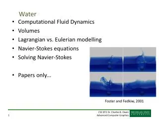
Water • Computational Fluid Dynamics • Volumes • Lagrangian vs. Eulerian modelling • Navier-Stokes equations • Solving Navier-Stokes • Papers only… Foster and Fedkiw, 2001
Computational Fluid Dynamics • CFD • Describes the characteristics of fluids in a volume • Animation vs. CFD • CFD – Initial conditions, let it run • Animation – Looks real and we have control • CFD – correctness • Animation – efficiency
Describing volumes • We need to describe the volume and what’s in it • Volumes are typically described using regular voxels (3D cells) (128 x 128 x 128 is common) • Boolean for each voxel Foster and Metaxas, 2000
Describing what’s in the volume • How do we describe water? • Ideas?
Two approaches • Derives from Computational Fluid Dynamics • Lagrangian models • What happens at points in space • Eulerian models • Where does stuff go
Lagrangian Models • Break space into volumes • Describe what is in each volume • Example: Incompressibility • What goes in must match what goes out
Eulerian Models • We track motion of actual things over time • Particles are usually used to represent water • Example: Incompressibility • Particles must adhere to some packing rule
Navier-Stokes equation • Describes the motion of incompressible fluids • Water, oil, mud, etc.
Divergence • u is the liquid velocity field • Operator is called the “divergence” operator. • Divergence of a vector field F, denoted div(F) or as above is a scalar field • When equal to zero (zero vector), we have a divergenceless field
Gradient vs. Divergence • I hate operator overloading
Divergenceless field • Implies incompressiblity • Mass is conserved • What goes out a point equals what goes in • Note: This is “inside” the water, not what happens when air mixes in
More equation parts Gravity and force viscous drag convection pressure pressure velocity viscosity density
Problems with Navier-Stokes • Acceleration is associated with moving elements, so Eulerian models make sense • Pressure and boundary conditions are at locations, so Lagrangian models make sense • Some methods use semi-Lagrangian models
Foster and Fedkiw method • 1. Model environment as a voxel grid • 2. Model liquid volume using particles and implicit surface • 3. Update velocity field by solving Navier-Stokes using finite differences and a semi-Lagrangian method • 4. Apply velocity constraints from moving objects • 5. Enforce incompressibility • 6. Update the liquid volume using new velocity field
The volume representation • Each cell has • Flag for filled or available for water • Pressure variable at center (optional) • Velocity vectors on 3 sides • Shared with adjacent cell
Particles • Water is represented by particles • Introduced from source or initially placed • Motion for particle is determined by tri-linear interpolation
Isocontour • Imagine each particle with a sphere around it Isocontour
Practical system issues • The isocontour is all we need for creating the image • High particle densities are needed to make good isocontours, but create lots of complexity • Create initial isocontour at high density, then use lower density motion fields to deform the isocontour • Other option: dynamically create/destroy particles
Solving Navier-Stokes • Step 1: Choose a time step • Good rule of thumb: Nothing can jump over any cells • ???
Solving • Step 2: Solve for the velocity • This is so much fun • Let w0(x) be a solution at location x at time t1 • We’ll move to a solution at time t2 using four steps
Getting to w1: Add force • w1(x) = w0(x) + Dt f
Getting to w2:Add convection • At each time step, all particles are moved by the velocity of the fluid • The particle at location x was at location p(x,t-Dt) before • Let w2(x)=w1(p(x,t-Dt)) • All that is required is a way to track particles and some linear interpolation.
Getting to w3:Viscosity • Can be shown that:
Finite differences • How do we get from or to code on arrays? • Finite differences:
Solving for viscosity This is a standard problem formulation called the Poisson Problem and can be solved using numerous solving packages like FISHPAK.
From FISHPAK C Subroutine POIS3D solves the linear system of equations C C C1*(X(I-1,J,K)-2.*X(I,J,K)+X(I+1,J,K)) C + C2*(X(I,J-1,K)-2.*X(I,J,K)+X(I,J+1,K)) C + A(K)*X(I,J,K-1)+B(K)*X(I,J,K)+C(K)*X(I,J,K+1) = F(I,J,K) C
Getting to w4:Incompressiblity • Our solution will have a divergence part and a divergence-free part. We need to solve for the divergence part and subtract it out.
Cont… Again, we have a Poisson Problem.
What about pressure? • Issues of incompressibility • Stam claims that pressure drops out in his solution. This would be a consequence of the way he deals with incompressibility.
Boundary conditions • What about where we run out of space? • Set velocity to zero? (paper says this) • Or what other option?