Download

1 / 56
560 likes | 663 Views
Bayesian Estimators of Time to Most Recent Common Ancestry. Bruce Walsh. jbwalsh@u.arizona.edu. Ecology and Evolutionary Biology. Adjunct Appointments Molecular and Cellular Biology Plant Sciences Epidemiology & Biostatistics Animal Sciences. Definitions.

E N D
Bayesian Estimators ofTime to Most Recent Common Ancestry Bruce Walsh jbwalsh@u.arizona.edu Ecology and Evolutionary Biology Adjunct Appointments Molecular and Cellular Biology Plant Sciences Epidemiology & Biostatistics Animal Sciences
Definitions MRCA - Most Recent Common Ancestor TMRCA - Time to Most Recent Common Ancestor Question: Given molecular marker information from a pair of individuals, what is the estimated time back to their most recent common ancestor? With even a small number of highly polymorphic autosomal markers, trivial to assess zero (subject/ biological sample) and one (parent-offspring) MRCA
Problems with Autosomal Markers Often we are very interested in MRCAs that are modest (5-10 generations) or large (100’s to 10,000’s of generations) Unlinked autosomal markers simply don’t work over these time scales. Reason: IBD probabilities for individuals sharing a MRCA 5 or more generations ago are extremely small and hence very hard to estimate (need VERY large number of markers).
MRCA-I vs. MRCA-G We need to distinguish between the MRCA for a pair of individuals (MRCA-I) and the MRCA for a particular genetic marker G (MRCA-G). MRCA-G varies between any two individuals over recombination units. For example, we could easily have for a pair of relatives MRCA (mtDNA ) = 180 generations MRCA (Y ) = 350 generations MRCA (one a-globulin allele ) = 90 generations MRCA (other a -globulin allele ) = 400 generations
MRCA-G( ) MRCA-G( ) lost MRCA-I MRCA-G > MRCA-I
mtDNA and Y Chromosomes So how can we accurately estimate TMRCA for modest to large number of generations? Answer: Use a set of completely linked markers With autosomes, unlinked markers assort each generation leaving only a small amount of IBD information on each marker, which we must then multiply together. IBD information decays on the order of 1/2 each generation. With completely linked marker loci, information on IBD does not assort away via recombination. IBD information decay is on the order of the mutation rate.
Y chromosome microsatellitemutation rates- I Estimates of human mutation rate in microsatellites are fairly consistent over both the Y and the autosomes
Basic Structure of the Problem What is the probability that the two marker alleles at a haploid locus from two related individuals agree given that their MRCA was t generation ago? Phrased another way, what is their probability of identity by state (IBS), given they are identical by descent (IBD) when their TMRCA is t generations
Infinite Alleles Model The first step in answering this question is to assume a particular mutational model Our (initial) assumption will be the infinite alleles model (IAM) The key assumption of this model (originally due to Kimura and Crow, 1964) is that each new mutation gives rise to a new allele. The IAM was the first population-genetics model to attempt to formally incorporate the structure of DNA into a model
A B (1-u)t (1-u) t Pr(No mutation from MRCA->A) = (1-u)t Pr(No mutation from MRCA->B) = (1-u)t MRCA MRCA Key: Under the infinite alleles, two alleles that are identical in state that are also ibd have not experienced any mutations since their MRCA. Let q(t) = Probability two alleles with a MRCA t generations ago are identical in state If u = per generation mutation rate, then q(t) = (1-u)2t
Building the Likelihood Function for n Loci - - - - - ( - ) - - For any single marker locus, the probability of IBS given a TMRCA of t generations is q(t) = (1-u)2t ≈ e-2ut = e-t, t = 2ut The probability that k of n marker loci are IBS is just a Binomial distribution with success parameter q(t) Likelihood function for t given k of n matches
( ) ( ) ^ - - ^ - ( - ) - - ML Analysis of TMRCA It would seem that we now have all the pieces in hand for a likelihood analysis of TMRCA given the marker data (k of n matches) Likelihood function (t = 2ut) MLE for t is solution of ∂ L/∂t = 0 p = fraction of matches
( ) - ( ) - - ^ - Var( t ) = ^ In particular, the MLE for t becomes Likewise, the precision of this estimator follows for the (negative) inverse of the 2nd derivative of the log-likelihood function evaluated at the MLE,
Finally, hypothesis testing, say Ho: MRCA = t0, is easily accomplished by comparing -2* the natural log of the ratio of the value of the likelihood function at t = t0 over the value of the likelihood function at the MLE t = t ^ Likewise, we can (numerically) easily find 1-LOD support intervals for t and hence construct approximate 95% confidence intervals to TMRCA The resulting log likelihood ratio LR is (asymptotically) distributed as a chi-square distribution with one degree of freedom
Trouble in Paradise The ML machinery has seem to have done its job, giving us an estimate, its approximate sampling error, approximate confidence intervals, and a scheme for hypothesis testing. Hence, all seems well. Problem: Look at k=n (= complete match at all markers). MLE (TMRCA) = 0 (independent of n) Var(MLE) = 0 (ouch!)
What about one-LOD support intervals (95% CI) ? With n=k, the value of the likelihood function is L(t) = (1-u)2tn ≈ e-2tun L has a maximum value of one under the MLE Hence, any value of t that gives a likelihood value of 0.1 or larger is in the one-LOD support interval Solving, the one-LOD support interval is from t=0 to t = (1/2n) [ -Ln(10)/Ln(1-u) ] ≈(1/n) [ Ln(10)/(2u) ] For u = 0.002, CI is (0, 575/n)
MLE(t) = 0 for all values on n 1 LOD ≈ t = 29 1 LOD ≈ t = 58 1 LOD ≈ t = 115 0.1 of max value (1) of likelihood function With n=k, likelihood function reduces to L(t) = (1-u)2tn ≈ e-2tun n=5 n=10 L(t) n=20 t (Plots for u = 0.002)
What about Hypothesis testing? Again recall that for k =n that the likelihood at t = t0 is L(t0) ≈ Exp(-2t0un) Hence, the LR test statistic for Ho: t = t0 is just LR = -2 ln [ L(t0)/ L(0) ] = -2 ln [ Exp(-2t0un) / 1 ] = 4t0un Thus the probability for the test that TMRCA = t0 is just Pr( c12 > 4t0un)
The problem(s) with ML The expressions developed for the sampling variance, approximate confidence intervals, and hypothesis testing are all large-sample approximations Problem 1: Here our sample size is the number of markers scored in the two individuals. Not likely to be large. Problem 2: These expressions are obtained by taking appropriate limits of the likelihood function. If the ML is exactly at the boundary of the admissible space on the likelihood surface, this limit may not formally exist, and hence the above approximations are incorrect.
posterior distribution of q given x Likelihood function for q Given the data x priordistribution for q The appropriate constant so that the posterior integrates to one. The Solution? Go Bayesian An extension of likelihood is Bayesian statistics Instead of simply estimating a point estimate (e.g., the MLE), the goal is the estimate the entire distributionfor the unknown parameter q given the data x p(q | x) = C * l(x | q) p(q) Why Bayesian? • Exact for any sample size • Marginal posteriors • Efficient use of any prior information • MCMC (such as Gibbs sampling) methods
The Prior on TMRCA The first step in any Bayesian analysis is choice of an appropriate prior distribution p(t) -- our thoughts on the distribution of TMRCA in the absence of any of the marker data Standard approach: Use a flat or uninformative prior, with p(t) = a constant over the admissible range of the parameter. Can cause problems if the likelihood function is unbounded (integrates to infinity) In our case, population-genetic theory provides the prior: under very general settings, the time to MRCA for a pair of individuals follows a geometric distribution
Prior hyperparameter = 1/Ne - - - - Previous likelihood function (ignoring constants that cancel when we compute the normalizing factor C) Prior In particular, for a haploid gene, TMRCA follows a geometric distribution with mean 1/Ne. Hence, our prior is just p(t) = l(1-l)t≈l e-lt, where l = 1/Ne Hence, we can use an exponential prior with hyperparameter (the parameter fully characterizing the distribution) l = 1/Ne. The posterior thus becomes
- - - - - - - - The Normalizing constant where I ensures that the posterior distribution integrates to one, and hence is formally a probability distribution
- - - - What is the effect of the hyperparameter? If 2uk >> l, then essentially no dependence on the actual value of l chosen. Hence, if 2Neuk >> 1, essentially no dependence on (hyperparameter) assumptions of the prior. For a typical microsatellite rate of u = 0.002, this is just Nek >> 250, which is a very weak assumption. For example, with k =10 matches, Ne >> 25. Even with only 1 match (k=1), just require Ne >> 250.
- - - - - ( - - - - = - - - - - - - - Closed-form Solutions for the Posterior Distribution Complete analytic solutions to the prior can be obtained by using a series expansion (of the (1-ex)n term) to give Each term is just a * ebt, which is easily integrated
- - - - - - - - - - - - - - - - - - With the assumption of a flat prior, l = 0, this reduces to
( - - - - - - - - - Hence, the complete analytic solution of the posterior is Suppose k = n (no mismatches) In this case, the prior is simply an exponential distribution with mean 2un + l,
< - - - - Analysis of n = k case Mean TMRCA and its variance: Cumulative probability: In particular, the time Ta satisfying P(t < Ta) = a is
For a flat prior (l = 0), the 95% (one-side) confidence interval is thus given by -ln(0.5)/(2nu) ≈ 1.50/(nu) Hence, under a Bayesian analysis for u = 0.02, the 95% upper confidence interval is given by ≈ 749/n Recall that the one-LOD support interval (approximate 95% CI) under an ML analysis is ≈ 575/n The ML solution’s asymptotic approximation significantly underestimates the true interval relative to the exact analysis under a full Bayesian model
n = 20, t0.95 = 38 n = 10, t0.95 = 75 Under a Bayesian analysis, we look at the posterior probability distribution (likelihood adjusted to integrate to one) and find the values that give an area of 0.95 Under ML, we plot the likelihood function and look for the 0.1 value Pr(TMRCA < t) n = 10, area to left of t=75 = 0.95 n = 20, area to left of t=38 = 0.95 t Why the difference?
Posteriors for n = 10 Posteriors for n = 20 Posteriors for n = 50 n = 100 93 n = 100 0.30 92 0.060 94 91 100 90 0.25 0.050 99 0.20 0.040 p( t | k ) p( t | k ) 98 89 0.15 97 0.030 96 95 0.10 0.020 0.05 0.010 0.00 0.000 1 2 3 4 5 6 7 8 9 10 11 12 13 14 15 16 17 18 19 20 0 5 10 15 20 25 30 35 40 45 50 55 60 65 Time t to MRCA Time t to MRCA Sample Posteriors for u = 0.002
Key points • By using markers on a non recombining chromosomal section, we can estimate TMRCA over much, much longer time scales than with unlinked autosomal markers • By using the appropriate number of markers we can get accurate estimates for TMRCA for even just a few generations. 20-50 markers will do. • Hence, we have a fairly large window of resolution for TMRCA when using a modest number of completely linked markers.
( - ] [ - - - Extensions I: Different Mutation Rates Let marker locus k have mutation rate uk. Code the observations as xk = 1 if a match, otherwise code xk = 0 The posterior becomes:
Mutation 1 Mutation 2 Under IAM, score as a match, and hence no mutations In reality, there are two mutations Stepwise Mutation Model (SMM) Microsatellite allelic variants are scored by their number of repeat units. Hence, two “matching” alleles can actually hide multiple mutations (and hence more time to the MRCA) The Infinite alleles model (IAM) is not especially realistic with microsatellite data, unless the fraction of matches is very high.
Y chromosome microsatellitemutation rates- II The SMM model is an attempt to correct for multiple hits by fully accounting for the mutational structure. Good fit to array sizes in natural populations when assuming the symmetric single-step model • Equal probability of a one-step move up or down In direct studies of (Y chromosome) microsatellites 35 of 37 dectected mutations in pedigrees were single step, other 2 were two-step
SMM0 model -- match/no match under SMM The simplest implementation of the SMM model is to simply replace the match probabilities q(t) under the IAM model with those for the SMM model. This simply codes the marker loci as match / no match We refer to this as the SMMO model
- - > - ( ) Formally, the SMM model assumes the following transition probabilities Note that two alleles can match only if they have experienced an even number of mutations in total between them. In such cases, the match probabilities become
- ( - The zero-order modifed Type I Bessel Function ( ) - Hence,
Under the SMM model, the prior hyperparameter can now become important. This is the case when the number n of markers is small and/or k/n is not very close to one Why? Under the prior, TMRCA is forced by a geometric with 1/Ne. Under the IAM model for most values this is still much more time than the likelihood function predicts from the marker data Under the SMM model, the likelihood alone predicts a much longer value so that the forcing effect of the initial geometric can come into play
n =5, k = 3, u = 0.02 IAM, both flat prior and Ne = 5000 SSMO, Ne = 5000 SSMO, flat prior Pr(TMRCA < t) Prior with Ne =5000 Time, t
> - The jth-order modifed Type I Bessel Function … … An Exact Treatment: SMME With a little work we can show that the probability two sites differ by j steps is just The resulting likelihood thus becomes Where nj is the number of sites that differ by k (observed) steps
… - - … - Number of exact matches Number of k steps differences With this likelihood, the resulting prior becomes This rearranges to give the general posterior under the Exact SMM model (SMME) as
Example Consider comparing haplotypes 1 and 3 from Thomas et al.’s (2000) study on the Lemba and Cohen Y chromosome modal haplotypes. Here six markers used, four exactly match, one differs by one repeat, the other by two repeats Hence, n = 6, k = 4 for IAM and SMM0 models n0 = 4, n1 = 1, n2 = 1, n = 6 under SMME model Assume Hammer’s value of Ne=5000 for the prior
IAM SMM0 P(t | markers) SMME Time to MRCA, t TMRCA for Lemba and Cohen Y
IAM SMM0 Pr(TMRCA < t) SMME Time to MRCA, t
Technology Transfer The expressions developed above have direct commercial applications Family Tree DNA (ftDNA) -- provides Y chromosome marker kits for genealogical studies So far, ftDNA has processed over 10,000 such kits This amounts to a rough gross of around 3 million dollars.
Forensic applications of the Y • A not uncommon situation is the only DNA is from fingernail scrappings. • The result is a mixture wherein the victim's DNA often overwhelms the DNA of the perpetrator. • Result: only modest match probability as many autosomal markers cannot be detected • One solution: use Y chromosome markers. Easily amplified over (female) background
Problem: How do we combine Y match with autosomal match? NRC 1996 recommendations (autosomal loci) Product rule across markers Population substructure correction within markers Prob(Y match)*Prob(autosomal match) Problem: Y markers may provide information about population substructure membership For example, a particular haplotype may be restricted to a certain subpopulation, e.g., Native Americans