Point Processing
Point Processing. Point by Point by Point. Taxonomy. Images can be represented in two domains Spatial Domain: Represents light intensity at locations in space Frequency Domain: Represents frequency amplitudes across a spectrum Operations can be classified as

Point Processing
E N D
Presentation Transcript
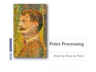
Point Processing Point by Point by Point
Taxonomy • Images can be represented in two domains • Spatial Domain: Represents light intensity at locations in space • Frequency Domain: Represents frequency amplitudes across a spectrum • Operations can be classified as • Point: a single input sample is processed to produce an output • Regional: the output is dependent upon a region of samples
Rescaling • Rescaling is a point processing technique that alters the contrast and/or brightness of an image. • Exposure is a measure of how much light is projected onto the imaging sensor. • An image is said to be overexposed if details of the image are lost because more light is projected onto the sensor than what the sensor can measure. • An image is said to be underexposed if details of the image are lost because the sensor is unable to detect the amount of projected light. • Images which are underexposed or overexposed can frequently be improved by brightening or darkening them. • In addition, the overall contrast of an image can be altered to improve the aesthetic appeal or to bring out the internal structure of the image. • Even non-visual scientific data can be converted into an image through adjusting the contrast and brightness
Rescaling • Given a sample Sinput of the source image, rescaling computes the output sample, Soutput, using the scaling function of 5.1 • Alpha is a real-valued scaling factor known as “gain” • Beta is a real-valued scaling factor known as “bias”
Rescaling • Consider two rescaled source samples S rescaled to S’. • Consider the contrast (difference) between them in both the source and destination. • Consider the relative change in contrast between the source and destination.
Rescaling • The relative change in contrast can be simplified as • Gain controls the change in contrast. Bias does not affect the contrast • Bias, however, controls the brightness of the rescale image. Negative bias darkens and positive bias brightens the image
Clamping • Rescaling may produce samples that lie outside of the output images 8-bit dynamic range. • May be less than zero • May be more than 255 • Clamping the output values ensures that the output samples are truncated to the 8-bit dynamic range limit • Any output greater than 255 is set to 255 • Any output less than zero is set to be zero • Clamping does ‘loose’ information by truncation
Examples gain = 1, bias = 55 gain = 1, bias = -55 gain = 2, bias=0 gain = .5, bias=0
Scientific Data and Visualization • Linear scaling is often used to map data that is not essentially visual in nature into an appropriate form for visual analysis. • A thermal imaging system, for example, essentially detects temperatures by sensing the infrared spectrum. The system may produce a two-dimensional table of temperature readings that indirectly correspond to a visual image but are in the wrong form for rendering.
Scientific Data • Consider the image of a dog on a hot summer evening. The range of temperatures might extend from 71.5 to 99.3 but these values don’t correspond well to visual data (it’s a mostly dark-gray image with little contrast). • The data can be rescaled to increase contrast enhance the visual interpretation of the data.
Contrast Stretching • If the goal of rescaling is to maximize the contrast of an image, then a precise selection of the gain and bias parameters is required. • Given a two-dimensional data set in the interval [a; b] the optimal gain and bias values for an 8-bit system are given below. • For color depths other than 8 the value 255 should be replaced by the largest sample value allowed in the destination image.
Rescaling Color Images • Rescaling can be naturally extended to color images by rescaling every band of the source using the same gain and bias settings. • It is, however, often desirable to apply different gain and bias values to each band of a color image separately. • Consider, for example, a color image that utilizes the HSB color model. Since all color information is contained in the H and S bands, it may be useful to adjust the brightness, encoded in band B, without altering the color of the image in any way. • Alternately, consider an RGB image that has, in the process of acquisition, become unbalanced in the color domain. It may be desirable to adjust the relative RGB colors by scaling each band independently of the others. • Rescaling the bands of a color image in a non-uniform manner is a straightforward extension to the uniform approach where each band is treated as a single grayscale image.
RescaleOp • Linear scaling is so common that Java contains a RescaleOp class for this purpose. • The constructor accepts three parameters • The gain (a float) • The bias (a float) • A RenderingHints object (usually null) • An example that uses this class is shown below’
RescaleOp • An alternate constructor allows for non-uniform scaling • The gain (an array of floats – one for each band) • The bias (an array of floats – one for each band) • A RenderingHints object (usually null) • An example that uses this class is shown below’ null); The textbook lists ‘src’ rather than ‘null’ as the third argument to the constructor. This is an error.
Lookup Tables • Rescaling can be performed with great efficiency through the use of lookup tables, assuming that the color depth of the source is sufficiently small. • Consider, for example, rescaling an 8-bit image. Without using lookup tables we compute the value clamp(gain*S+bias, 0, 255) for every sample S in the input. • For an WH image there are WH samples in the input and each of the corresponding output samples requires one multiplication, one addition, and one function call. • But note that since every sample in the source must be in the range [0, 255] we need only compute the 256 possible outputs exactly once and then refer to those pre-computed outputs as we scan the image. • Lookup tables are effective when the color depth is not too great and the complexity of the filtering operation is large enough.
Lookup Tables • In an 8-bit image, for example, each sample will be in the range [0, 255]. Since there are only 256 possible sample values for which the quantity clamp( gain * S + bias, 0, 255) must be computed, time can be saved by pre-computing each of these values, rather than repeatedly computing the scaled output for each of the WH actual input samples. • These pre-computed values are stored in a lookup table.
Lookup Tables • Lookup tables will generally improve the computational efficiency of rescaling (although integer-based arithmetic ops may outperform tables in some cases). • Lookup tables are flexible. The rescaling operation represents a linear • relationship between input and output sample values but a lookup table is able to represent both linear and nonlinear relationships of arbitrary complexity. • Java’s image processing library contanis a LookupOp class. • The LookupOp is a BufferedImageOp that must be constructed by providing a LookupTable object. The LookupTable object is a thin wrapper for an array of bytes.
LookupOp and LookupTable • An example of how to use Java’s lookup operations is shown below:
Gamma Correction • Gamma correction is an image enhancement operation that seeks to maintain perceptually uniform sample values throughout an entire imaging pipeline. • In general terms, an image is processed by (1) acquiring an image with a camera, (2) compressing the image into digital form, (3) transmitting the data, (4) decoding the compressed data, and (5) displaying it on an output device. • Images in such a process should ideally be displayed on the output device exactly as they appear to the camera. • Since each phase of the process described above may introduce distortions of the image it can be difficult to achieve precise uniformity. • Gamma correction seeks to eliminate distortions introduced by the first and the final phases of the image processing pipeline.
Gamma Correction • Cameras and displays possess intrinsic physical properties that introduce non-linear distortions in the images they produce/display. • For a display, the non-linearity is best described as a power-law relationship between the level of light that is actually produced and the amount of light that is intended to control the display. • This relationship is given below where gamma is the controlling parameter. This formulation assumes normalized samples in the range [0, 1].
Gamma Correction • Gamma describes the amount of distortion • Gamma value of 1 means no distortion • Computer monitors typically have gammas of 1.2 to 2.5 • Since most displays introduce a distortion of the intended image, pre-processing is used to remove the distortion. • This pre-processing is called “gamma correction” and is given by 5.8.
Gamma Correction • Consider the effects of gamma correction on the intended image as it is displayed. • Gamma correction can be encoded in a digital file format. • Example: PNG supports gamma correction since it allocates the “gAMA” chunk that “specifies the relationship between the image samples and the desired display output intensity”. This value can the be used in pre-processing steps.
GammaOp implementation • Gamma correction can be implemented as a specialization of the LookupOp. • The constructor simply makes a LookupUp using a special LookupTable.
Gamma Correction • Most graphics cards/monitors have gamma settings • Values typically range from 1.8-2.5 [usually 2.2] • PCs typically have higher gamma settings than Macs so images typically look darker on PCs than Macs 3.0 2.5 2.0 1.5
Pseudo (False) Coloring • A pseudo-colored image is one that renders its subject using a coloring scheme that differs from the way the subject is naturally perceived. • While the term pseudo signifies false or counterfeit, a pseudo-colored image should not be understood as an image that is defective or misleading but as an image that is colored in an unnatural way. • While rescaling is able to maximize grayscale contrast, it is often desirable to render the image using a color scheme that further enhances the visual interpretation of the data.
Pseudo (False) Coloring • Consider the thermal image of a dog. The grayscale version is a contrast-stretched version of the original scientific data. The color version is pseudo-colored to enhance understanding.
Pseudo (False) Coloring Implementation • False coloring takes a source image (typically a gray-scale source) as input and produces a true-color image as output by replacing each gray-scale level by an arbitrary palette color. • There are at most 256 colors in an image that has been pseudo colored from an 8-bit grayscale source. • The most natural fit for this operation is the indexed color model since the palette will contain at most 256 colors. • Can construct an IndexColorModel object (part of the Java library) by supplying three arrays each of which represents the red, green and blue samples.
Custom Pseudo (False) Coloring Implementation using an array of Colors