Download

1 / 30
300 likes | 333 Views
Learn about confidence intervals, t-tests, F-tests, and regression analysis in analytical chemistry to analyze and compare data effectively.

E N D
Example: Daily level of an impurity in a reactor has a mean 4.0 and = 0.3. What is the probability that the impurity level on a randomly chosen day will exceed 4.4? Applications Tail = 0.0918 or ~ 9%
The more times you measure a quantity, the more confident that the average of • your measurements is close to the true population mean. • Uncertainty decreases in proportion to , where n is the number of measurement
4-2 Confidence intervals Confidence interval: Interval within which the true value almost certainly lies!
Confidence Limit: How sure are you? • In equation 4 - 6 t is a statistical factor that depends on the number of degrees of freedom (degrees of freedom = N-1). • n is the number of measurements Values of t at different confidence levels and degrees of freedom are located in table 4.2
Exercise 4A: For the numbers 116.0, 97.9, 114.2, 106.8 and 108.3, find the mean, standard deviation, and 90% confidence interval for the mean. • Solution: the mean = (116.0 + 97.9+ 114.2+106.8+108.3)/5 = 108.64 the standard deviation s = … the t value from Table 4-2 is: 2.132 use equation 4-6 to calculate the confidence interval:
The meaning of a confidence level • Standard deviation is frequently used as the estimated uncertainty. • It is a good practice to report the number of measurement so that confidence level can be calculated
4-3 Comparison of Means with Student’s t • Confidence limits and the t test assume that data follow a Gaussian distribution. If they do not, different formulas would be required. • t test can be used to compare whether two sets of measurements are “the same”, i.e. whether the observed difference between the two means arises from purely random measurement error. • We customarily accept the result if we have a 95% chance that the conclusion is correct.
Case 1: Comparing a measured result with a “known” value • Computing the 95% confidence interval for your answer and check if that range includes the “known” answer. • If the known answer is not within the 95% confidence interval, the results do not agree.
A reliable assay shows that the ATP (adenosine triphosphate) content of a certain cell type is 111 μmol/100 mL. You developed a new assay, which gave the following values for replicate analyses: 117, 119, 111, 115, 120 μmol/100 mL (average = 116.4). Can you be 95% confident that your result differs from the “known” value? The 95% confidence interval does not include the accepted value of 111 μmol/100 mL, so the difference is significant.
Case 2: Comparing replicate measurements • Lord Rayleigh’s experiments: the discovery of Argon. • For two sets of data consisting of n1 and n2 measurements with averages , calculate a value of t with the formula • Find t in Table 4-2 for n1+ n2 -2 degree of freedom. If tcalculate >Ttable(95%), the difference is significant
Case 3: Pared t test for computing individual difference • Situation: using two methods to make single measurements on different samples, i.e. no measurement has been duplicated. • To see if there is a significant difference between the methods, one uses paired t test.
T = 2.228 for 95% CI Related: Problems: 4.1 to 4.4 and 4.7, 4.17, 4.19 to 4.22.
4-4 Comparison of standard deviations with the F test • If the standard deviations of the two data set are significantly different, then the following equation is needed for the t test. • The F test tells us whether two standard deviations are significantly different from each other.
F = s12/s22 • Use degrees of freedoms 1 and 2 to find a F value from Table 4-4. • If the calculated F value exceeds a tabulated F value at a selected confidence level (95%), then there is a significant difference between the variances of the two methods. • Problem 4-17. If you measure a quantity 4 times and the standard deviation is 1.0% of the average, can you be 90% confidence that the true value is within 1.2% of the measured average.
4-6: Rejection of a Result:The Q Test • The Q test is used to determine if an “outlier” is due to a determinate error. If it is not, then it falls within the expected random error and should be retained. • Q = gap/w where gap = difference between “outlier” and nearest result and w = range of results. • If Qcalculate > Qtable, the questionable point should be discarded.
4-7: The method of least squares (Regression Analysis) The straight line model Starting point: Line through the origin Experience suggests that there is an error in the response, therefore,
The method of least squares takes the best fitting model by minimizing the quantity, A plot of S as a function of Beta produces a minimum with a constant least square estimate for beta “m”. After “m” is known, you have all the calculated values The difference between these two values is the residual, and the sum of the squares of the residuals is also a minimum value.
Estimate of the experimental error variance, s2 The coefficient of determination R2 is the proportion of variability in a data set that is accounted for by a statistical model. The version most common in statistics texts is based on analysis of variance decomposition as follows: